6 Supply
In this chapter you will learn:
- Understand different cost concepts
- Be able to explain economies and diseconomies of scale
- Be able to explain profit maximization in a competitive market
- Be able to explain that the supply curve is the marginal cost curve
- Describe causes for shifts in the supply curve
6.2 Cost concepts
We will begin with definitions of fundamental concepts of cost. This might be a bit dry, but it is crucial.
Fixed costs, \(FC\): are all those costs that are independent of how much stuff is produced and sold.
- An example of a fixed costs at a University is the landscaping budget. How many tulips planted every year surely is independent of how many students enroll or how many academic papers get published at IU.
Variable costs, \(VC\): are all these costs that are dependent on how much stuff is produced and sold.
- The more students that are enrolled the more Covid-19 testing units need to be available.
Total costs, \(TC\): are just fixed costs plus variable costs, \(FC + VC\)
If we now let the quantity \(q\) denote the amount or quantity produced, then we can define:
Average fixed costs, \(AFC = \frac{FC}{q}\).
Average variable costs, \(AVC = \frac{VC}{q}\).
Average total costs, \(ATC = \frac{TC}{q}\).
Marginal cost, \(MC\): is the extra cost incurred to produce one more unit.
Average fixed cost is easily graphed as in Figure 6.1. The fact that this is downward sloping and slowly approaches 0 should not be a surprise. This is just an application of “the big-little principle40” from middle school. Since fixed costs do not depend on quantity produced, as we are increasing quantity over the x-axis we are spreading the fixed costs out more and more over a larger quantity (denominator for AFC).
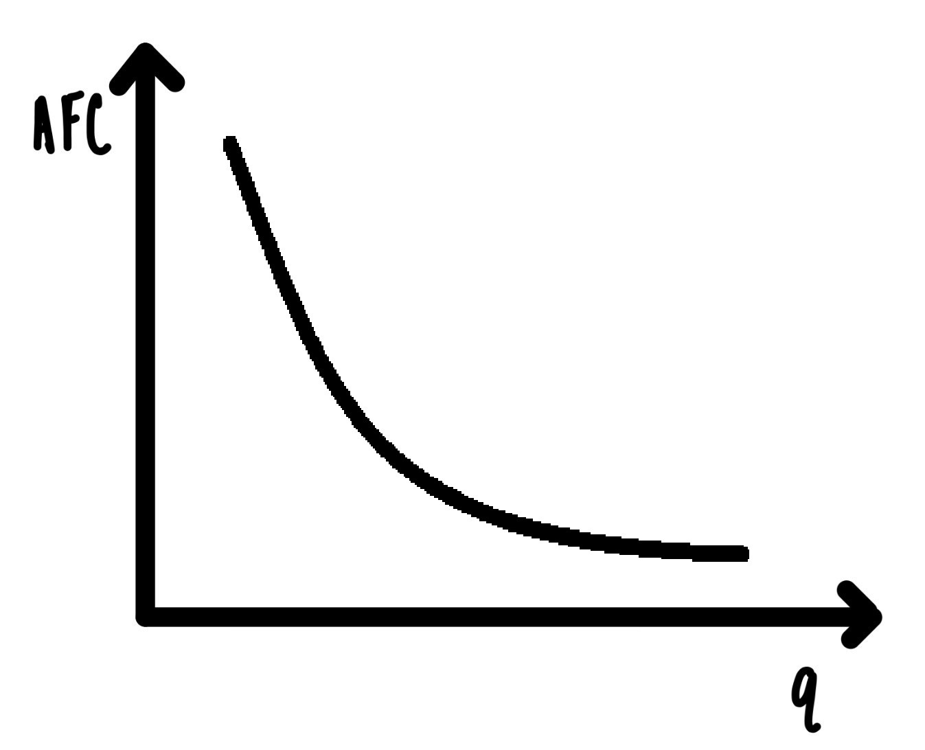
Figure 6.1: Average Fixed Costs
6.3 Economies of Scale
Production costs vary in often fundamental ways across industries. We have many industries that are dominated by a few very large firms. And we have many industries where there are lots and lots of rather small firms.
Good place to add in some examples of different industries varying in sizes. We could then link it to the example industries throughout the section
What might cause this difference?
In some industries we will find economies of scale or increasing returns to scale. We will use these two terms interchangeably.
When there are economies of scale, it is cheaper, on average, to produce on a large scale than on a small scale. The average costs decline as more output is produced. That means that the average cost curve is downward sloping. There are increasing returns to scale.
In other industries there are diseconomies of scale. When there are diseconomies of scale, it is more expensive, on average, to produce on a large scale than on a small scale. The average costs increase as more output is produced. That means that the average cost curve is upward sloping. There are decreasing returns to scale.
When there are economies of scale, it is cheaper on average to produce on a large scale. Then we should expect few large firms. When there are diseconomies of scale, it is cheaper on average to produce on a smaller scale. Then we would expect many, many smaller firms in this industry.
In many cases when we look at an individual firm, we would expect economies of scale to prevail at low levels of production and, eventually, as more and more output is produced economies of scale give way to diseconomies of scale. That means that at low levels of output, the average cost curve is downward sloping and at high levels of output, the average cost curve is upward sloping, making the average cost curve U – shaped.
Figure 6.2 illustrates this U-shaped average cost curve. To the left of the figure there are economies of scale or increasing returns to scale, indicated by the abbreviation, IRS. To the left of the figure there are diseconomies of scale, or decreasing returns to scale, indicated by the abbreviation DRS.
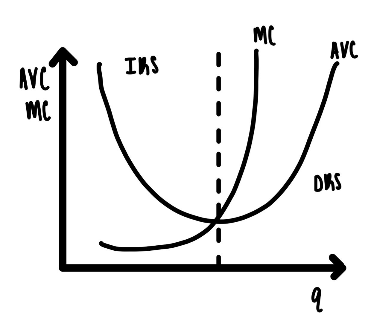
Figure 6.2: Average Variable Cost and Marginal Cost.
Figure 6.2 also shows the marginal cost curve, MC. As indicated in the figure, the MC curve is below the average variable cost curve, when AVC is declining and MC is above the AVC curve when AVC is increasing. This has to be like that. For proof, see exercises 1-3 at the end of this section.
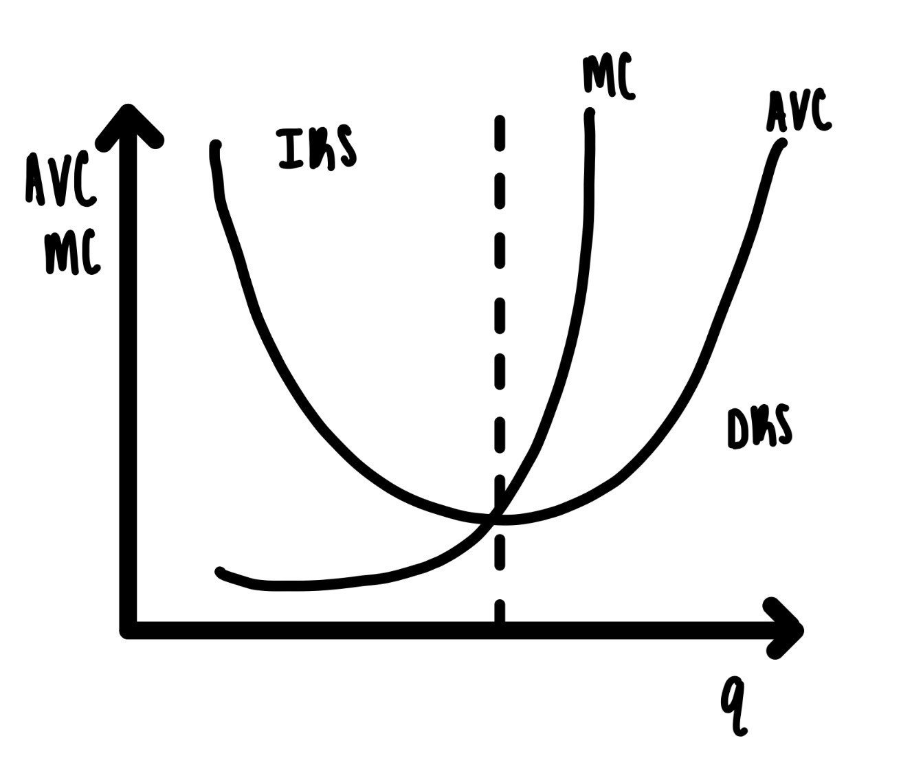
Figure 6.3: Average Variable Cost and Marginal Cost
It follows, that the MC curve must intersect the AVC curve at the bottom of the AVC curve. If the MC curve intersected the AVC curve at any other spot, the MC curve would be above and below the AVC curve when the AVC curve is declining. In Figure 6.3 the MC curve intersects the AVC curve at a place where AVC is declining. If you look at the area inside the red circle, the AVC curve is downward sloping everywhere in the red circle, but the MC curve is below on the left and above on the right in the red circle. We know this is non-sense.
After the cases in increasing returns to scale and the case of decreasing returns to scale there is one important benchmark case to consider: The case of constant returns to scale.
After the cases of increasing returns to scale and the case of decreasing returns to scale, there is one important benchmark case to consider: the case of constant returns to scale. Constant returns to scale, CRS, are present when the average cost of production is constant regardless of the amount of output produced. In this case, the average cost curve is a horizontal line as indicated in Figure 6.4. In Figure 6.4 the marginal cost curve and the average cost curve coincide. This makes sense, if the marginal cost of making a t shirt is \(\$3.80\) for each and every shirt, then the average cost is also \(\$3.80\).
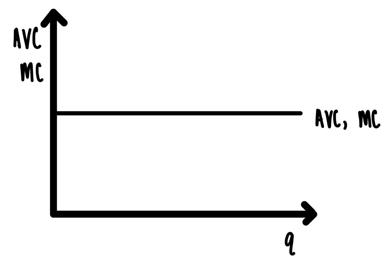
Figure 6.4: Constant returns to scale.
6.3.1 Examples
When we look around, we can see decreasing returns and increasing returns in action. When the production technology is characterized by decreasing returns, average cost curves are downward sloping, it is more expensive on average to produce large quantities and less expensive to produce small quantities. If that is so and if firms are concerned with minimizing costs, we would then expect many firms in a market, each producing relatively small amounts. Here we are some examples of industries/markets where we typically see many small firms:
Barber Shops
Tattoo Parlors
Restaurants
Nail Salons
Craft Breweries
In these cases we suspect that the technology exhibits decreasing returns.
On the other hand, when there are increasing returns, average cost curves are downward sloping, and it is cheaper on average to produce large quantities. Then we would expect large firms and since the firms are large, there would be few in number. Examples would include:
Pharmaceutical Companies
Power Companies
Insurance Companies
For pharmaceutical companies, the lions’ share of the cost is up front costs of R&D. Often that reaches into the hundreds of millions of dollars. These costs need to be spread out over many doses sold. The more doses are sold, the lower the average total cost of a dose is.
In all of the above discussion, the increasing or decreasing returns, whether the average cost curves are upward or downward sloping always depends on up the size of the relevant market, whether relevant demand is large or small.
Bloomington, IN hospital has 278 staffed beds. That seems puny relative to the size of the country. But that is beside the point. Bloomington Hospital is intended to only serve Bloomington and the immediately surrounding areas. Here we are talking about a potential market size of perhaps 150,000 people. That hospital with fewer than 300 beds is plenty big, relative to its market.
6.4 Profit Maximization
We will study profit maximization in a competitive market. The definition of a competitive market, as in chapter 3, is: all participants in the market are price takers, or at least act as if they were price takers.
A few years ago, during a visit of Plymouth, MA, I went to a quaint little seafood market and restaurant and struck up a conversation with the daughter of the owner about the seafood market in Plymouth. Just about the very first thing she said was: “Of course, we can’t raise the price.”
Why not?
If you ever been to Plymouth or similar little cities, you will know that there are seafood markets and restaurants everywhere. If one market raises the price of lobster, people will go elsewhere.
“Of course, we can’t raise the price.” This is just expressing that they know they operate in a competitive market.
So how does profit maximization work in a competitive market? Jack, the owner of the Halibut Hut, knows he can sell a pound of halibut at $15 per pound. Jack also knows the marginal costs of catching halibut. How much halibut should he catch? The answer is in Figure 6.5.
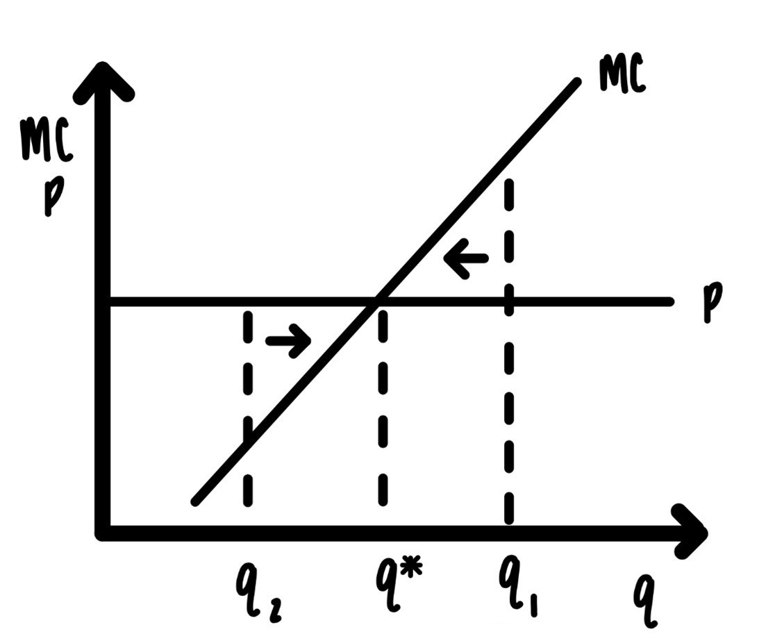
Figure 6.5: Constant returns to scale.
The claim is: In order to maximize profit Jack should catch halibut so that the marginal cost of catching halibut is exactly equal to the price. In Figure 6.5, if the price of halibut is given by \(p\), then the profit maximizing quantity is given by \(q^*\).
If Jack sold less, say \(q_2\). At \(q_2\) the price is above marginal cost. Selling one extra unit generates more revenue than it costs to produce that unit. Profit maximization requires that Jack produces more, which is indicated by the arrow pointing right.
At \(q_1\), the marginal cost is above the price. Jack is losing money on that last unit. He should not produce it. He should produce less, which is indicated by the arrow pointing left.
Punchline:
If the price is p, the profit maximizing quantity is q*.
Profit maximization in a competitive market requires that MC = p.
6.5 Supply
Figure 6.6 shows how we can get from profit maximization to supply. Profit maximization says:
If the price is \(p_1\), sell \(q_1\).
If the price is \(p_2\), sell \(q_2\).
Etc
As the price changes profit maximization sweeps along the marginal cost curve. At any price dictated by the market, the marginal cost curve determines through profit maximization, how much the firm will produce. This allows us to call the marginal cost curve the supply curve. In other words:
The supply curve IS the marginal cost curve.
There is one additional wrinkle: If the price falls too low, below the minimum average cost, then the firm will not be able to cover its cost. In this case it will have to go out of business and produce zero units of output. So, if you look at Figure 6, the supply curve consists of two parts. The first part is just the marginal cost curve where marginal cost is above the average cost curve. The second part is the vertical axis when output is zero when the price is below average costs. This is indicated by the dashed line in Figure 6.6.
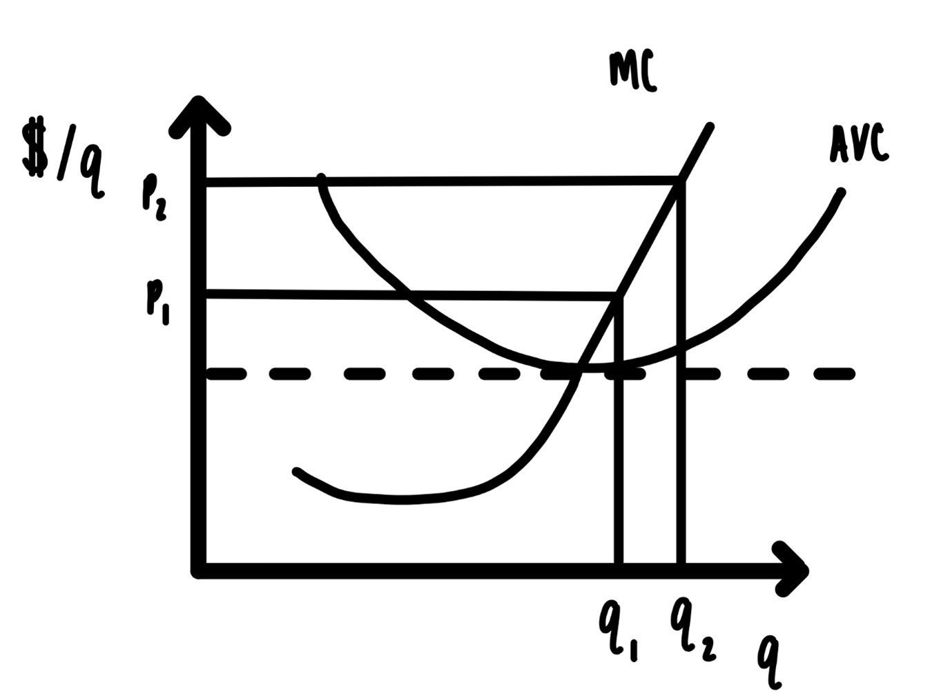
Figure 6.6: Average variable cost and marginal cost.
6.6 Shifts in Supply
There are many factors that can shift the supply curve. The first, and over the long run probably most important, factor is technological progress. When technological progress lowers marginal costs, the supply curve shifts down vertically or, equivalently, it shifts to the right (horizontally). This represents an increase in supply as indicated in Figure 6.7.
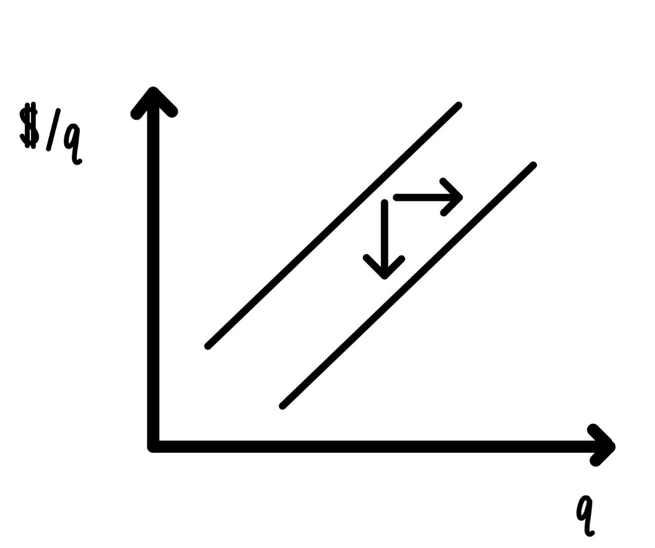
Figure 6.7: Technological progress.
One example of tremendous technological progress is called Moore’s law. This is illustrated in Figure 6.8. It basically says that computing power on a chip doubles every 2 years. From Figure 6.8, it is apparent that that law has been in place since the 1970s. There you see the incredible power of exponential growth.

Figure 6.8: Technological Progress Example: Moores Law
In Figure 6.9 we can see that the costs of solar panels have fallen from over $75 to less than 40 cents per watt.
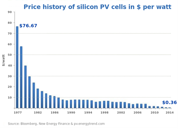
Figure 6.9: Technological Progress Example: Solar Panelsd.
Nordhaus (1996)41 has documented that the cost of light, measured in lumens, has experienced a similarly drastic fall over the last 200 years (Figure 6.10 below)
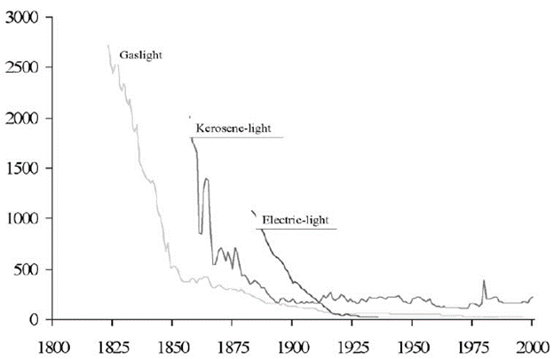
Figure 6.10: Technological Progress Example: Solar Panels.
Of course, there are also forces that can increase marginal costs, and thus, decrease supply, i.e., shift supply to the left. If there is an increase in the minimum wage, the marginal cost of production will rise to the extent that the costs of labor are variable costs. If the government imposes extra safety regulations that increase marginal costs, then supply will decrease or shift to the left. If the price of gasoline rises, the supply of rides by Lyft, Uber or cabs decreases. Such a leftward shift in supply is indicated in Figure 6.11.
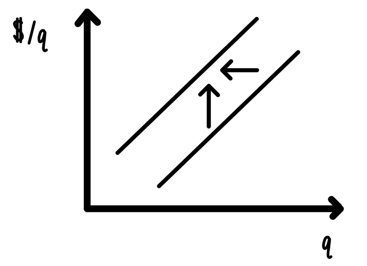
Figure 6.11: Increase in marginal cost.
6.7 Glossary of Terms
Average fixed costs: Fixed costs divided by the total amount of output.
Average variable costs: Variable costs divided by the total amount of output.
Constant returns to scale: Constant returns to scale are present when the average cost of producing is independent of the total amount of output produced.
Decreasing returns to scale: Decreasing returns are present when average costs of producing are increasing as more output is produced.
Diseconomies of scale: The same as decreasing returns to scale.
Economies of scale: The same as increasing returns to scale.
Fixed costs: That part of cost which is independent of the total amount of output produced and sold.
Increasing returns to scale: When the average cost of producing are decreasing as more output is produced.
Marginal costs: The extra cost incurred of producing one more unit.
Profit: Total revenue minus total costs
Supply: The set of points that indicate how much output a profit-maximizing firm sells in a competitive market al all-possible prices. The marginal cost curve.
Technological progress: A change in technology, typically generated by R&D, that can lower marginal costs.
Total costs: The sum of fixed costs and variable costs.
Total revenue: The price of the product multiplied by the amount of the product sold.
Variable costs: That part of cost that does depend on the total amount of output produced and sold.
6.8 Practice Questions
6.8.1 Discussion
Imagine a quarter back playing six games. These are his pass completions for these six games: 52%, 49%, 48%, 46%, 45%, 43%. For the first one, two, three, four, five, six games calculate average completion rates. There will be six averages. Graph these six averages together with the performance on the last game.
Imagine a basketball player who scores the following number of points in six games: 12, 10, 10, 9, 7, 6. Calculate and graph the six average and marginal performances.
Imagine a running back who in six games has the following yardage: 54, 62, 63, 68, 75, 80. Calculate and graph the six average and marginal performances.
Imagine a 400-meter runner who has six races over a season with the following times in seconds: 58, 56, 56, 57, 58, 58. Calculate and graph the six average and marginal performances.
Collect date for average or median income for the 50 states for the year 2000. Also collect data for these states and for the same year for population size. Put both sets of observations on a scatter plot with population size going on the horizontal axis and the income measure on the vertical axis. Judging from your scatter plot, do you think there are increasing, constant or decreasing returns to scale when each state is considered as a production unit with labor/people as an input and median/average income as an output?
Repeat exercise 6 for European countries.
Repeat exercise 6 for Latin American countries.
For a local clothing store like Mirth Market on Kirkwood make a list of at least 6 items that contribute to fixed cost and a list of at least 6 items that contribute to variable cost.
For the store in exercise 8, define marginal cost.
-
Please read this article on airline food.
- Make a list of all the items required to make tasty airplane means that would contribute to Fixed Cost.
- Make a list of all the decisions that have to be made to provide tasty airline that were/are surprising to you.
6.8.2 Multiple Choice
-
If a firm in a competitive market operates where marginal cost is above the price, then the firm should
A. Increase output
B. Decrease output
C. Keep output constant
D. Sell the plant to the German -
If a firm in a competitive market operates where marginal cost is below the price, then the firms should
A. Increase output
B. Decrease output
C. Keep output constant
D. Buy more plants from the Canadians -
If a firm in a competitive market operates where marginal cost is equal to the price, then the firm should
A. Increase output
B. Decrease output
C. Keep output constant
D. Sponsor Nascar -
If fixed costs increase, then the entire supply curve
A. Shifts to the right
B. Shifts to the left
C. Stays constant
D. Becomes steeper -
If an industry is characterized by diseconomies of scale, then we would expect in that industry
A. A few very large firms
B. Many very small firms
C. A mixture of small and large firms
D. Elon Musk to own at least 50% of all firms -
If an industry is characterized by constant returns to scale, then we would expect in that industry
A. A few very large firms
B. Many very small firms
C. A mixture of small, medium and large firms
D. Prices to be high -
In a competitive industry we would expect
A. That firms take the price as given
B. That there are a few firms that dictate the price
C. Each firm to produce where the price is above marginal cost
D. Each firm to produce where the price is below marginal cost -
When average costs are downward sloping, we would expect marginal costs
A. To be above average costs
B. To be below average costs
C. To be horizontal
D. To be vertical -
When average costs are U-shaped, there are
A. Economies of scale at low levels of production and diseconomies of scale at high levels of production
B. Diseconomies of scale at low levels of production and economies of scale at high levels of production
C. Constant returns to scale
D. Economies of scale for all levels of production -
When average costs are U-shaped, then marginal costs
A. Intersect average costs where average costs are upward sloping
B. Intersect average costs where average costs are downward sloping
C. Intersect average costs where average costs are minimized
D. Are also U-shaped -
If fixed costs decrease, then
A. Variable costs decrease
B. Total costs decrease
C. Marginal costs decrease
D. Average variable costs decrease -
Moore’s Law is an example of
A. Economies of scale
B. Diseconomies of scale
C. Constant returns to scale
D. None of the above -
If the price increase, a competitive firm will
A. Produce more
B. Produce less
C. Experience a shift to the right of the supply curve
D. Experience a shift to the left of the supply curve -
If the price drops below minimum average costs, a competitive firm will
A. Produce more
B. Produce less
C. Produce zero
D. Not change its production -
A competitive firm will
A. Take the price a given
B. Act as price taker
C. Be unable to influence the price
D. All of the above -
Imagine Jack owns a plant in Columbus, IN that makes ball bearings. Jack builds a new plant to make ball bearings in Kokomo, IN. Production in the second plant exactly duplicates all inputs from the Columbus plant. All prices of inputs are the same in Columbus and Kokomo. Then we would expect costs in Kokomo to be
A. Higher than in Columbus
B. Lower than in Columbus
C. The same as in Columbus
D. Astronomical -
The thought experiment in question 16 illustrates
A. Economies of scale
B. Diseconomies of scale
C. Constants returns to scale
D. Competitive markets -
In the production of electricity, we would expect
A. Economies of scale
B. Diseconomies of scale
C. Constant returns to scale
D. Many small firms -
In the “therapeutic massage industry”, we would expect
A. Economies of scale
B. Diseconomies of scale
C. Constant returns to scale
D. A few large firms -
Imagine a firm in a competitive market. Suppose that its marginal cost curve shifts down, then we would expect
A. The price to rise
B. The price to fall
C. Its quantity supplied to rise
D. Its quantity supplied to fall