4 Decisions: Rational or Irrational?
In this chapter you will learn:
- The basics of a simple model of rational choice
- The concepts of marginal costs and marginal benefits
- The concept and applications of opportunity cost
- The concept of diminishing returns
- The concept of increasing returns.
4.1 Goals and Constraints
In this section we will construct our workhorse model/theory that we will use in the rest of the term. We will learn about the notion of rationality that is commonly used in economics. We will learn what rationality means and we will learn what choices are like if they are governed by rationality.
Rationality always begins with the assumption of a goal or of an objective. We assume that all of our behavior is guided by goal, that all of our behavior is purposeful or goal oriented. Our goals will vary from person to person. There is no reason to believe that your goals should be the same as my goals. We simply accept whatever goals individuals might have. And we do not judge them. We recognize that our individual goals may vary from time to time.
Leslie’s goal is to get elected to Congress. Jack’s goal is to graduate from IU with at least a 3.7 grade point average with a major in economics and a minor in computer science. George’s goal is to slay the dragon. Georgina’s goal is to be able to retire at age 49 with a retirement portfolio valued at least at 4 million dollars.
Our goals can change overtime. As Georgina realizes at age 40 that she is far away from her goal she might adjust her goal of retiring to age 55. Sometimes we set aside some goals completely and work on other goals almost exclusively.
Joanne wants to be valedictorian in her high school. She is a varsity soccer player. During the soccer match on Saturday afternoon, she does not even think about her English project or her chemistry lab; she only thinks about the soccer match. During those 90 minutes her goal of being valedictorian does not enter her mind at all; the only thing that matters to her in those 90 minutes is winning the game.
In pursuit of our goals, we are typically limited by a variety of constraints:
First: There is a budget or financial constraint. That 10 million dollar mansion in Malibu overlooking the Pacific is not in my budget. Nor is the luxurious trip around the world in 180 days. Most of us are facing this type of budget constraint. Perhaps if you are Elon Musk you don’t feel it as much as the average IU student.
Second: Most of us face time constraints. There are only 24 hours in a day. Sometimes these time constraints are more binding, or at least they feel more binding than at other times. If we go on a nice vacation with our family, hanging out at the beach, watching the waves gently lap on the sandy beach, time seems to stand still, there is no rush and we might well ask: A time constraint? What is that? But our life is not like that all of the time. Just think of the parents who are rushing to fill out their tax forms late on April 14th. That is crunch time. Or think of your own situation as you are preparing for four difficult final exams while two projects are due and while the university is asking you to move out of your dorm room within 36 hours of your last exam. That is also crunch time. Then the time constraint bites, it really bites.
Third: Most of us are facing constraints that have to do with our intellectual bandwidth. How much can we compute or calculate? How many hundreds of pages can we read over the weekend for a project in our history class and fully comprehend what we read? Evidently, in chess one secret to success is to be able to figure 8, 10, 12, or 15 moves ahead including how the adversary will respond to each one of our moves. Some of us have that gift, that large bandwidth. I certainly don’t.
Fourth: Many of us in some points in our lives will face emotional constraints. People experiencing poverty often live in the tyranny of the moment, going from one crisis to another. The mom with two young children who has struggled all her life to make ends meet and who just found out that her husband has abandoned her might well be at the end of her rope and ask: how much more can I take? She is facing severe emotional constraints.
Some constraints are technological. They just say that certain things are physically impossible. One of my dreams has been to climb Kilimanjaro, but I think I have to face the fact that at my age and in my physical condition that is impossible. There are many such a technological constraint.
A nice example of such a technological constraint is illustrated in Figure 1 below. It is recognized that between 1960 and 2010 computing power has doubled every two years. That sounds like a fantastic achievement. That is just Moore’s Law.
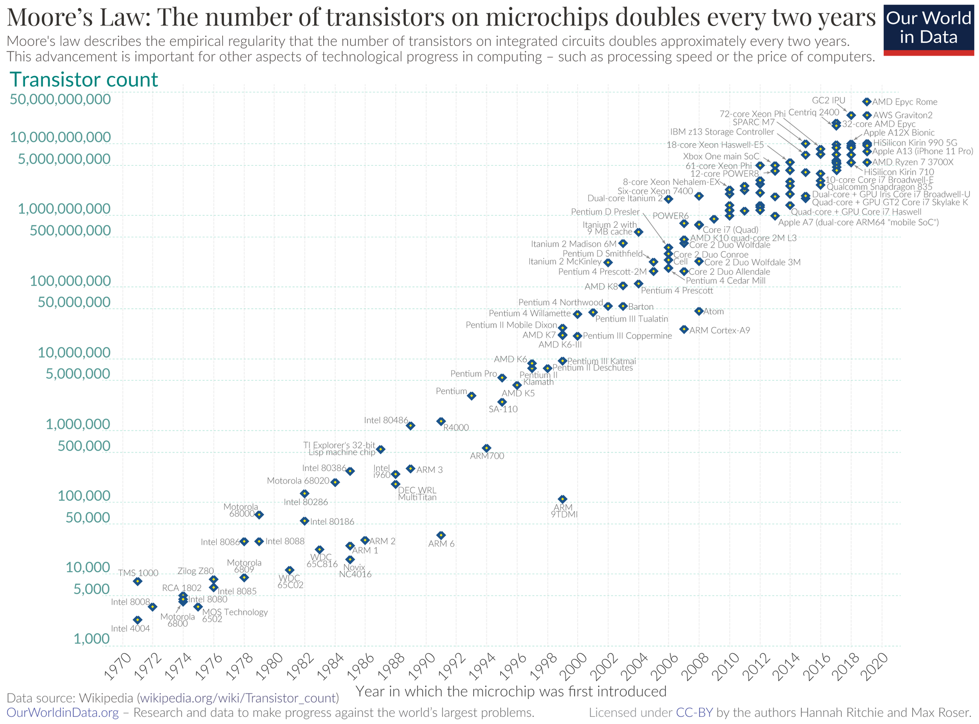
Figure 4.1: Moores Law
It turns out that for some purposes the doubling of computing power every two years is not enough. In order to train systems of artificial intelligence, AI, well, a doubling of computing power every 3 to 4 months seems to be required. Good luck with speeding up the growth of computing power by a factor of 6!
Figure 4.2: Source: The Economist, “The cost of training machines is becoming a problem” July 13, 2020.
4.2 Marginal Costs and Benefits
We will now illustrate the foundations for a model of rational choice. Whenever we make a choice we weigh, if we are rational, the costs of the action and the benefits of the action. We will start with an action that can be chosen in small increments.
Examples of such actions are:
- How many miles do I want to hike this coming weekend?
- How much money do I want to contribute to a charity?
- How much time do I want to spend texting my parents while I’m getting ready for my exam in college?
- How much time do I want to study for the final in my introductory economics course?
- How much chocolate do I want to eat this week?
In all of these cases, the choice is a continuous variable, the choice is not a discrete, all or nothing kind of choice.
Of course, there are many choices that are of the all-or-nothing variety:
- Getting on an airplane to fly to San Diego during Covid-19: yes or no?
- Attending IU: yes or no?
- Marrying my high-school sweetheart: yes or no?
In a sense, the all or nothing choices are relatively easy to model and understand. If you think you are better off marrying your high school sweetheart than not, then, by all means, marry your high school sweetheart. In econ speak: if the benefit of marrying your highschool sweetheart exceeds the cost, then go ahead and marry your high school sweetheart. (Of course, it takes two to tango!)
The decisions where continuous choices are involved might be somewhat harder to model. This is what we are embarking on now. We need some terminology.
The marginal benefit of an action, MB, is the extra benefit obtained by carrying out the action one more unit.
The marginal benefit of hiking one extra mile is the enjoyment I get out of being in nature for another 20 to 30 minutes or so. And, of course, it is the extra calories I burn by hiking one extra mile so I can eat more cookies when I get home.
The marginal benefit of studying for the exam in my economics class is the extra understanding of the material I gain, and it includes the increased probability that I ace the exam.
The marginal benefit of talking to my mom on the phone for an extra half-hour is simply the enjoyment of communicating with my mom and it could include some extra probability of getting my allowance increased.
The marginal cost of an action, MC, is the extra cost incurred by carrying out the action one more unit.
The marginal cost of hiking one extra mile includes a bunch of things. In that extra time, 20 or 30 minutes, I could be doing all kinds of other things, like sitting on my back porch and eating cookies. If I hiked an extra mile, I might get so tired that I lose concentration, stumble over a rock or a root, fall and break an ankle. If I hiked an extra mile, I run an extra risk of getting lost and I might not be able to get back home on time for an important appointment.
The marginal cost of studying an extra hour for the exam in my economics class includes not studying for the exam in my chemistry class and it includes things like watching TV or hanging out with my friends.
The marginal cost of communicating with my mom on the phone includes not studying for my economics exam.
You get the idea. If I commit sometime to one particular action, there are a whole bunch of other things I cannot do at the same time. If I donate $100 to one charity, I cannot donate it to another charity. If Jose works in industry 1, he cannot work in industry 2.
This brings us to the notion of opportunity cost.
Opportunity cost is one of the most important concepts in economics, if not the single most important one, and it is crucial that we have a firm grasp off this concept.
The definition of opportunity cost is simply: the value of the next best alternative forgone by making a particular choice.
Let’s consider the following possibilities ranked in order pleasure or utility I derive from them:
- reading a good book
- reading the New York Times
- reading a letter from my son
- going for a walk
- talking to my brother on the phone
- cleaning the gutters on my roof
And there are many others. If these are really listed in order of priority and importance for me, I will choose reading a good book.
What is the opportunity cost of reading a good book? It is not the pleasure I get out of talking to my brother on the phone. That is the fifth best thing I could be doing at that moment. The opportunity cost of reading a good book is reading the New York Times. Reading the New York Times is my next best alternative after reading a good book. So, the opportunity cost of reading a book is the value I would have derived from reading the New York Times, my second-best alternative forgone.
4.3 Choice
We will now present our basic and simple model/theory of rational choice. We make two assumptions.
Assumption 1: The marginal benefit of an action, MB, is declining as the action is increased.
When we graph the marginal benefit of an action it will be downward sloping. In Economics this assumption is known as
Diminishing returns or Diminishing utility
This is an assumption, not a universal law, that makes sense in many situations, but not in all. We will address some exceptions later on. But in many situations, this makes sense.
After cutting grass in my backyard on hot Saturday in July, the first sip or glass of sweetened iced tea just tastes great and quenches my thirst. The second glass a little bit less, the fourth glass not so much.
That first hour of a hike on a mild fall day feels wonderful. By the third hour I feel tired and my back hurts from carrying a backpack.
Seeing a boyfriend/girlfriend for the first time after a long separation can feel like heaven. After a few days/weeks, the routine has set in, the elation and excitement are gone.
Example 1: A few years ago, there was a solar eclipse that could be seen mid-afternoon, with the proper protective glasses, of course. I remember feeling very excited about stepping out of my building on the way to class with my protective gear. Seeing the eclipse was stunning, truly stunning. I just kept looking and looking. But after three or so minutes, the excitement had warm off. Diminishing returns had set in in my case. Evidently, something very similar had happened to most of the IU students I saw along the way. The administration had made allowances for the students to be out of class so they could watch the eclipse. Huge numbers of students were outside. They were outside, but were they enthralled by the eclipse? Evidently not. Most of them were just chatting with each other, ignoring the eclipse. Their diminishing returns had set in even before mine.
Example 2: Pricing for Disney theme parks in Florida also displays an example of diminishing returns. In this case the diminishing returns refer to the pleasure Mickey Mouse fans may experience from visiting the Magic Kingdom. On the Disney website you can purchase tickets for visits between 1 and 10 days. Wow, 10 days in the Magic Kingdom! What magic!
Here are the total prices for tickets for 1 to 10 days, at least as of 08/18/21.
| # of Days | Total Price | Difference per Day |
|---|---|---|
| 1 | 109 | 105 |
| 2 | 214 | 101 |
| 3 | 315 | 97 |
| 4 | 412 | 28 |
| 5 | 440 | 10 |
| 6 | 450 | 19 |
| 7 | 469 | 19 |
| 8 | 488 | 16 |
| 9 | 504 | 16 |
| 10 | 520 | 16 |
Evidently, there is a large drop after day 4. Why? If the marginal benefit of the ninth day were as high as the marginal benefit of the second day, surely Disney would change its pricing scheme.
Assumption 2: The marginal cost of an action, MC, is increasing as the action is increased.
The graph of marginal cost is upward sloping.
This also goes by the name of diminishing returns.
This is also an assumption, not a universal law. In many cases this assumption rings true.
Imagine studying for a chemistry exam the night before the exam. You have not really kept up well with the material in that class and you know you will have to study way past midnight to have a shot at doing well. You start studying right after dinner at 7 pm. The mental effort required to learn is higher at midnight than at 10 pm and at 10 pm it is higher than at 8 pm. Your consumption of coffee or power drinks goes up as time goes on.
Studying each chapter gets harder and harder the longer you study. The effort required to understand a given chunk of material goes up over time. The marginal cost of acquiring knowledge rises. That is diminishing returns.
We can now put together the marginal benefit of an action and the marginal cost of the action. This is done in Figure 2. Let a, on the horizontal axis, denote the extent of the action. MB and MC of that action are graphed on the vertical axis. For the sake of concreteness, assume we are talking about how long Leslie should study for her chemistry exam.
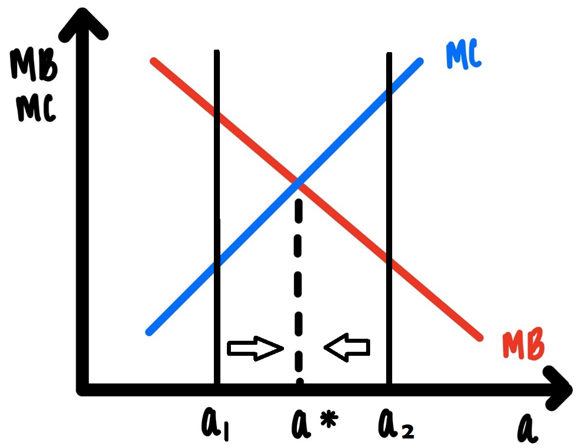
Figure 4.3: Rational Choice,
In Figure 4.3, the marginal benefit of the action, MB, is downward sloping in accordance with assumption 1. The marginal cost of the action, MC, is upward sloping in accordance with assumption 2.
Claim: The optimal amount of time Leslie should study for the chemistry exam, IF Leslie is rational, is given by a*.
Why? Imagine that Leslie did anything else. Imagine she studied less, only \(a_1\). At that point, the marginal benefit of studying an extra half hour exceeds the marginal cost. So, Leslie should study an extra half hour. She should study more. She should move from \(a_1\) to the right closer to a* as indicated by the arrow pointing right. If Leslie is rational, she will do just that.
Imagine Leslie studies more, say \(a_2\). At that point, the marginal cost of studying that last half hour exceeds the marginal benefit. Sleep deprivation does not usually translate in high exam scores. At \(a_2\) Leslie should decide to study less. She should move to the left, as indicated by the arrow pointing left. Rational Leslie will do just that.
We have established in the case of Leslie studying for her exam, but much more generally:
Rational action requires that the marginal benefit of an action is equated to the marginal cost of an action.
This conclusion which is illustrated in Figure 4.3 above will provide the basis for about 80% of the material in this class. Figure 4.3 will show up in this class, again and again, just in different contexts.
In Figure 4.3, the marginal benefit curve is downward sloping, and the marginal cost is upward sloping. We will encounter three versions of Figure 4.3 in this course. They are just very slight variations of Figure 4.3. These are depicted in Figure 4.4. Panel a is just a reproduction of Figure 4.3. In panel b, the marginal benefit curve is a horizontal line, and the marginal cost is upward sloping. In panel c, the marginal benefit is downward sloping, and the marginal cost is a horizontal line.
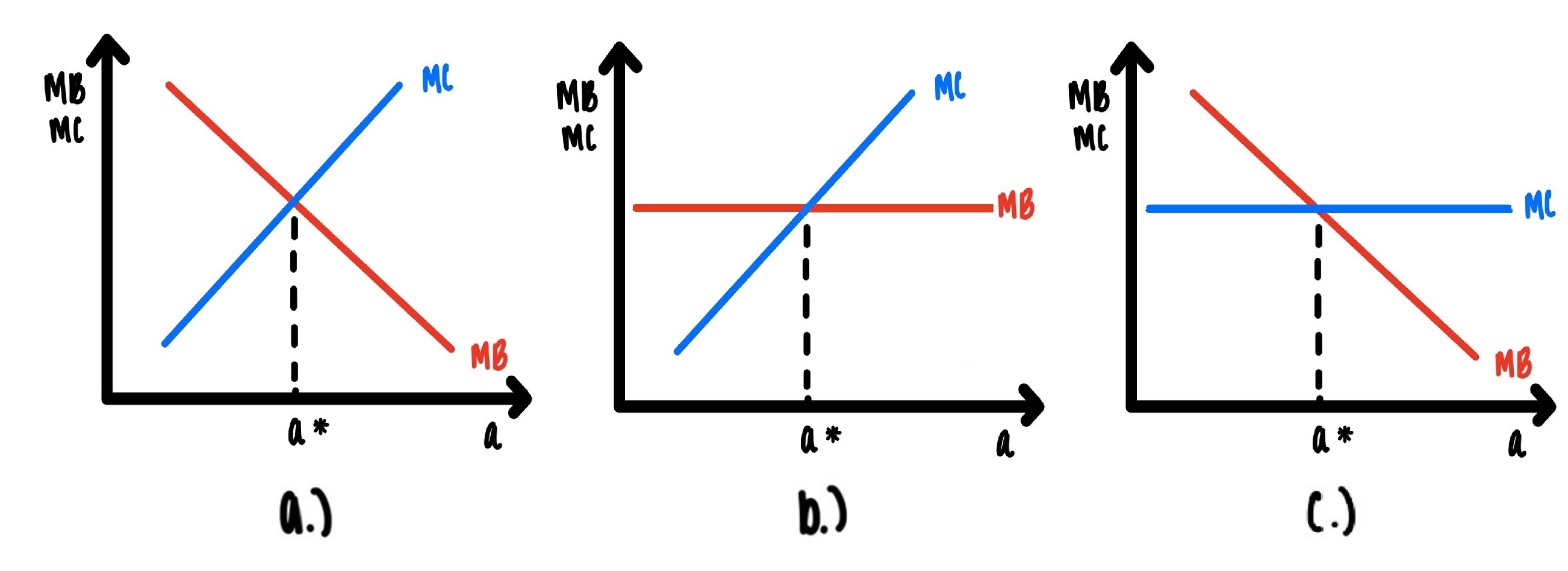
Figure 4.4: This photo will reappear many times!
We can get from panel a to panel b by rotating the marginal benefit curve downward, so it becomes horizontal. We can get from panel a to panel c by rotating the marginal cost downward, so it becomes horizontal.
While these panels look slightly differently, they are just slightly different versions of the same thing:
At low levels of the activity, marginal benefit is above marginal cost. At high levels of the activity, marginal cost is above the marginal benefit. Somewhere in between there is a sweet spot, where marginal benefit equals marginal cost.
4.4 Changes in Marginal Benefit and/or Marginal Cost
What if some event occurs in which the marginal benefit or cost of an action changes?
The environment in which we live is not static. Our circumstances change all the time. In the framework laid out above there will be frequent changes in the marginal benefits and the marginal costs for our actions. How do these shifts influence rational action?
In Figure 4.5 we show how an increase in the marginal benefit of the action changes our rational choice.
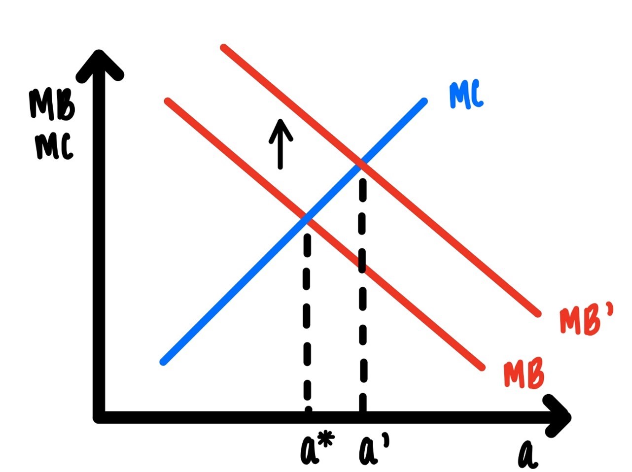
Figure 4.5: Increase of Marginal Benefit
Imagine that you are planning on a 3-hour hike by yourself this coming Saturday. Saturday morning your best friend calls you up and tells you he has nothing to do that day. You are overjoyed and invite him on the hike. Hiking with your best friend is much more enjoyable than a solitary hike. Because your friend accompanies you on your hike, the marginal benefit curve shifts out (Figure 4.5) to the right. As a consequence, your 3-hour hike turns into a 4-hour hike. That is the rational response.
In Figure 4.6 we show how an increase in marginal cost of the action changes your rational choice.
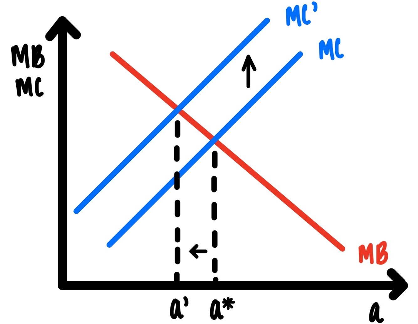
Figure 4.6: Increase of Marginal Cost
Imagine you are planning a 3-hour hike for this coming Saturday. Saturday morning your wake up and you realize that overnight there was torrential rain that turned the hiking trails in your area into mud. Each step is a muddy slog. Each step now is drudgery. The rain has increased the marginal cost of hiking (Figure 4.6). Your 3-hour hike turns into a 2-hour hike. That is the rational response.
4.5 Examples of Rational Choice
Example 3 (Refreshing Lemonade): You just cut the grass on a hot July afternoon. You are hot, sweaty, and parched. Figure 4.7 captures the marginal benefit and the marginal cost of drinking lemonade. Assume the units of measurement are small glasses. The marginal cost of drinking lemonade is just the cost of each glass of lemonade. It is the same for each small glass. It is a horizontal line. The marginal benefit declines with each glass. The first glass is a great thirst quencher and so is, perhaps the second glass. Glasses three and four less so. By the sixth glass the marginal benefit is tiny, below marginal cost. It is rational for you to drink 4 glasses.
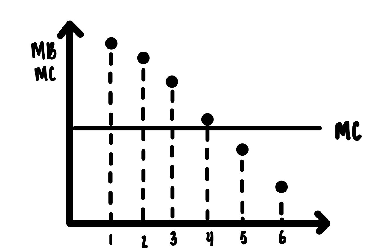
Figure 4.7: Drinking lemonade on a hot Saturday afternoon after you cut the grass.
Example 4 (Optimal Retirement): Joe is a dedicated high school math teacher. He has been teaching for 38 years and he has been planning to teach until his 70th birthday. After careful consideration of the joys of teaching, the marginal benefit, and the costs, this was his optimal choice. He has noticed that in the last few years, it has become harder to get up with a spring in his step every morning, and it has become harder to concentrate while grading papers. Yet, he still likes his job, with the joys outweighing any negative considerations. Then Covid-19 hit. Online teaching, lack of resources, concern for his health, administrative back and forth, administrative indecision, and opinionated parents who seem to stand in the way of effective teaching. This has caused his marginal benefit to shift way down. Now, retirement at age 67 instead of age 70 looks very appealing, and rational. It appears, nurses are in the same storm.
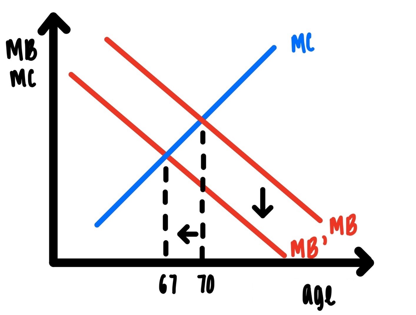
Figure 4.8: Optimal retiring age.
Example 5 (Optimal Family Size): What is our optimal number of kids? I know the number of children is not a continuous variable like how long to hike or how long to study for an exam. We still can imagine that there is a marginal benefit from having children and a marginal cost. Let’s assume for the sake of simplicity that the marginal cost of a child is constant. I know that things like hand me down clothes might make the second child cheaper than the first, but this will not matter for the argument here. I also know that some parents look forward to having several children, rather than just one to see their children play with each other and grow up with each other. One could make therefore an argument that the marginal benefit of the second child might be higher than the marginal benefit from child number 1. Again, this would not influence the argument here. The point is that eventually the marginal cost of an extra child is higher than the marginal benefit of that child. One interesting fact about desired fertility in the US seems to be: Whatever the number of children, if there is no boy among these children, the probability of having another child goes up. Suppose that for child 3, the marginal benefit is just above the marginal cost. Then the optimal rational number of children is 3. But things don’t stop here. The sex composition of children seems to matter for the decision to have another child. If all three previous children are girls, indicated by the string (G, G, G), then the marginal benefit of having a fourth child is high, above marginal cost and the family has a fourth child. If there is at least one boy among the first three, indicated by the potential strings (B, G, G), (G, B, G), (G, G, B), (B,B, G), (G, B, B), then the marginal benefit of a fourth child is low. The family will only have three children.
That’s the theory. That is also in the data. https://econweb.ucsd.edu/~gdahl/papers/demand-for-sons.pdf
American families tend to have a preference for sons over daughters.
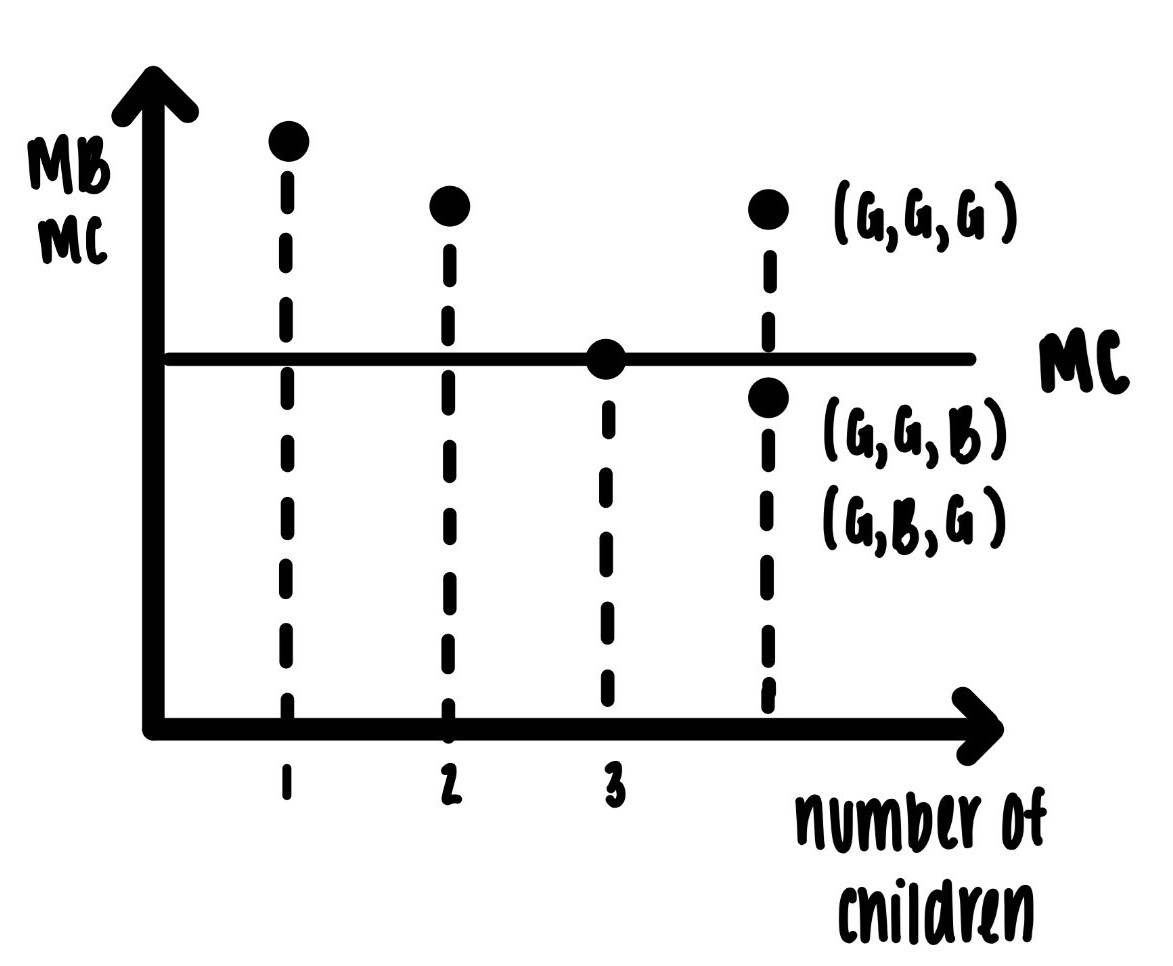
Figure 4.9: Optimal fertility
4.6 Increasing Returns
We said earlier that diminishing returns is not an iron law. It is an assumption that is helpful in many cases. We have seen some examples above. There are cases where there are not diminishing but increasing returns.
Example 6: Suppose you want to build a bridge over the Mississippi just north of St. Louis. It will require a ton of concrete. The point of the bridge is to get more transportation services from IL to MO and back. The marginal cost of the concrete can be assumed to be constant as seen in Figure 4.10.
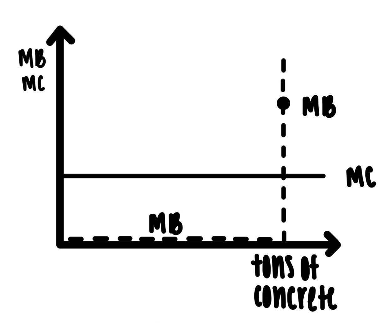
Figure 4.10: Concrete for bridge
The marginal benefit derived from the concrete is the shape of an inverted L. It is basically zero for practically every ton of concrete. There will be no transportation services at all until the very last ton of concrete is used to complete the bridge. Only when the last ton of concrete is laid, will there be any transportation services. Hence the inverted L shape.
Example 7: Suppose a widow, mother of two young children, is \(\$750\) behind on utilities. If she cannot pay the utility bill by next week, the power company will disconnect her service. Apart from not being able to heat the apartment and cook, disconnect from the power company means loss of her Section 8 housing and she and her two children will be homeless. Joe is a generous soul and gives her \(\$200\). That helps just a little bit, but her utility will still be shut off and she still faces the prospect of homelessness with her kids. Generous Jill pitches in another \(\$200\), and so does generous Jacqui. The marginal benefit of each one of these contributions is relatively small, since even with \(\$600\) she still faces the prospect of homelessness. Generous Jack finally pitches in another \(\$200\). This helps her over the top. It might be reasonable to assume that the marginal benefit to the widow of these contributions is as indicated in Figure 4.11, convex at first, below the $750 threshold and concave on the other side.
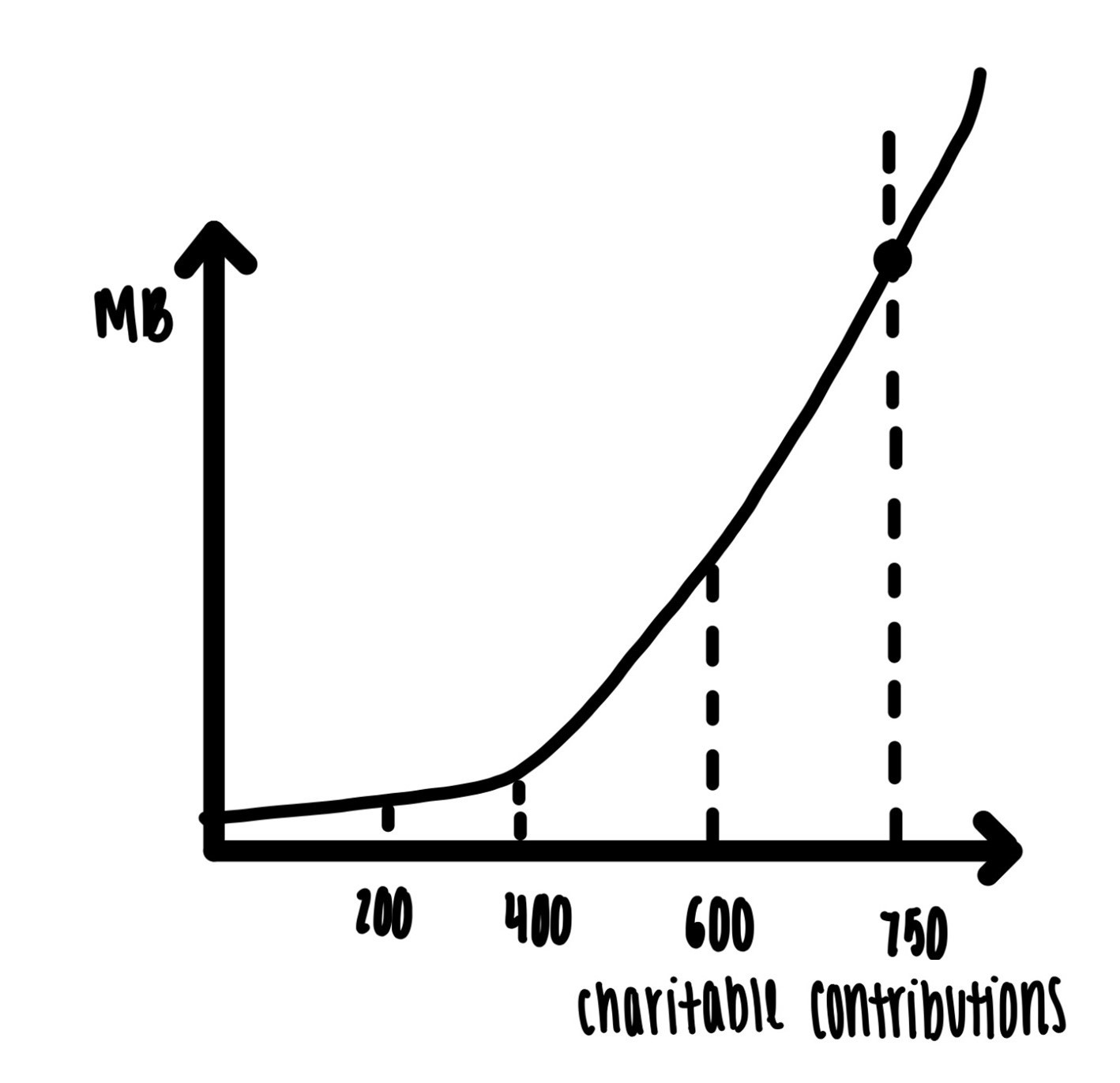
Figure 4.11: Benefit to widow of charitable contributions
Example 8: Why do you go to school? When I ask students that question the answer is invariably: To get a better job. And when I ask: What is a better job? the answer very often is something like: More money. The connection between schooling, years of schooling, and wages or earnings is one of the age-old central topics in labor economics.34

Figure 4.12: Source: Cecilia Elena Rouse, 2017, The economics of education and policy: Ideas for a principles course, The Journal of Economic education, 48:3, 229-237
The return to an extra year of schooling is basically zero between 1 and 11 years of schooling. If you are in high school and contemplating whether you want to drop out after 9th grade or whether you want to stick it out for one more year, the data seem to indicate that the monetary return to the 10th year is zero. If you are in it for the money, it is better to finish high school.
After high school, earning rise linearly with each extra year of schooling. Even past 16 years of schooling. So, you may want to make the effort to really finish college and perhaps even get a graduate degree. Good luck with that!
4.7 Irrationality
In the examples we have studies so far, we have always assumed that individuals make rational choices. Rationality means doing one’s best to attain one’s goal or goals, given the information we have and staying within our constraints.
There is quite a bit of evidence that not all decisions are rational. Many of the examples of irrational behavior involve a time dimension of either costs or benefits of the decision. Most of us have been there and have seen some indication of what irrational behavior might be: New Year’s rolls around and we resolve to start jogging and lose 20 pounds. But by March we have not jogged a mile, have not set foot in a gym, and forget about losing the 20 pounds. From eating all the chocolate, we have gained weight, not lost it.
Sometimes we just want to get one small snack, like one small piece of that delicious Swiss chocolate. So, we get the chocolate bar, break off one small piece, which is after all, all we want. But before we know it, the entire bar is devoured. And then regret sets in right away: Why did I eat so much chocolate? Why was I so stupid to eat the whole bar?
4.7.1 Sunk Costs
You get tickets for a Drake concert at the end of the month. You shell over the $200 for the tickets. The morning of the concert, your girlfriend whom you love above all else, surprises you with a text message. She informs you that she finished her studies abroad at the London School of Economics early, that she is back in town and that she can’t wait to spend the evening with you. You have missed her so much. Just the day before, before you saw the text, you told your body you would spend a thousand bucks to be with her. It is now too late to try to sell the Drake tickets on the secondary market.
What should you do? Most textbooks would say: You value the evening with your girlfriend more than going to the concert. The 200 bucks are sunk, they are a sunk cost. There is nothing you can do to retrieve the 200 bucks. Let
“Bygones be bygones”,
forget about the cost of the tickets and enjoy the evening with your girlfriend. Most econ text tell stories like that, give examples like that and then conclude that if you let sunk costs decide your behavior that you are engaged in what they call the
Sunk cost fallacy.
The Sunk cost fallacy says: You are not acting rationally of you let the size of the sunk costs, irretrievable costs incurred in the past, influence your current behavior.
But if that is all they say, their analysis is at least incomplete.
Letting sunk costs influence our current behavior might actually be quite rational. In the first counter example we will see that financial constraints will making a difference here.
Consider a firm with a budget of \(B\) dollars. The firm is engaged in an investment project that has a rate of return of \(R_1\). That project requires a fixed cost of \(M_0\) dollars. The firm is making payments on this project in some increments over time. At some point, after having made some payments in the amount \(M_1\) on project 1, the firm discovers a new project that is better in the sense that it has a higher rate of return \(R_2 > R_1\). The new project has the same fixed costs \(M_0\).
If \(M_1 < M_0\), then the firm rationally switches to project 2 if and only if
\((B – M_0) R_1 < (B – M_0 – M_1) R_2\)
It is easy to see that it is rational for the firm to switch to project 2 when B is large. But when B is small, i.e., when the firm faces a financial constraint, it will be rational for the firm to stay with the first project, EVEN THOUGH THE SECOND PROJECT IS BETTER.
Here is a more concrete example:
“…an aircraft company that had started a project to develop a radar-blank bomber plane might seem overly reluctant to switch to developing a radar-blank fighter plane if stealth fighters are suddenly in much greater demand; but their reluctance might be rational because they might have a limited budget, might have already spent hundreds of millions of dollars on developing a cost-effective bomber, and would have to pay another large fixed cost to develop a cost-effective fighter instead.”
So much for the sunk cost fallacy in this context. It is rational to “throw good money after bad money”.
The sunk cost fallacy may fall apart for other reasons as well. Some of these have to do with information and reputation.
Consider a manager who chooses a project. The manager is acting as the agent for the stockholders, the principals. Of course, the stockholders do not have perfect information about the quality, the ability of the manager. They infer ability of the agent from actions and outcomes.
While the project is being carried out, the manager acquires some information about the project. That information is typically private to the manager; the stockholders do not have access to the information. How are projects chosen? Hard to say, but it stands to reason that high ability managers choose high return projects more frequently than low ability managers might.
If a manager abandons a project, stockholders, the principal, might draw negative inferences about the manager’s ability. The manager of course has an interest in avoiding such an inference because that would negatively impact future earnings potential. For this reason, it is often rational for a manager to continue funding an unproductive project. Letting “bygones be bygones” may not be rational for him. The simple version of the sunk cost fallacy does not apply here. Even if the project is ultimately declared a failure with the manager being fired because of that failure, delaying that firing as long as possible may well be the most rational thing for the manager to do.
So much for the sunk cost fallacy in this context. It is rational to “throw good money after bad money”. The problem of rationally throwing good money after bad money may even be intensified in the political context. If I know there is a good chance that I will not be re-elected at the next election in two or four or six years, then, if I know the current project has turned out to be a lemon, I have a very large incentive of throwing good money after bad, so that the outcome of my bad decisions can be blamed not on me, but on my successor.
4.7.2 Examples
Example 9 (Gym membership, we don’t sweat it, but perhaps we should.):35
Gym member ship typically comes in three varieties: annual memberships, monthly memberships and daily passes. Prices in the sample in the paper above are approximately $12 per day, between about $85 per month for the monthly membership, and about $850 for an annual pass. Typically, you sign up for one of these options and then, after you signed one of these contracts, you go to the gym.
Or not.
That is exactly the issue studied in this paper by Stefano DellaVigna and Ulrike Malmenidier.
How would we think of rationality in this context? Rationality here implies that the choice of contract is consistent with actual exercise behavior. Signing up for a monthly contract is in your best interest if you actually go to the gym more than 7 times a month. (7 times 12 is 84) If you go to the gym fewer than 7 times a month, the daily memberships would have been a better deal. Similar comparisons can be made to decide on the rationality of choosing between the monthly and the annual contracts.
Here is what the authors find in their sample of over 7,700 individuals:
Those who choose a monthly contract pay on average 70% more relative to the daily contracts. How can this happen? Go 4 times a month. Using the daily passes costs $48. The monthly pass costs $85. (85-48)/48 = 37/48 = 77%.
The number of people overpaying like this is large. 80% of all customers would have been better off with the daily passes rather than the monthly contract.
Consumers who use the monthly contracts are 17% more likely to stay beyond one year than users of the annual contracts, even though using the monthly contract is more expensive in that case.
What is going on? It appears that most customers are naïve and over-estimate their future self-control. Looks like rationality has gone out the window.
These kinds of irrational behaviors often happen when there is a time or temporal element involved, which surely is the case in the choice of picking gym membership contracts.
Choose the contract today, and exercise in the future. Or not.
This is similar in many ways to:
Trip to the Dairy Queen today and the expectation of starting a jogging regimen in the future. But then the jogging does not happen. The benefits of the ice cream are today, the costs come in the future. And with the costs might come regrets. Why did I have that ice-cream?
The pleasure of smoking today and lung cancer at age 62. Regrets?
The costs of going to college today and the benefits of higher earnings over the entire productive life. Are there any regrets of not having worked hard enough in college?
Hooking up and enjoying the pleasure of sex tonight. The pleasure comes tonight, the potential costs in the future. The regret may set in already the following morning. The STDs may set in later and last a long time. By some estimates 1 in 2 people will contract a STI by age 25. The risk of getting infected during a hook up is substantial. 14% of male college students report 4 or more sexual partners in the last 12 months. For women in college that number is 9%. In a hookup, who is your partner? What is the risk? The three quarters of college students who report zero or one sexual partner probably present a smaller risk of infection, but they are probably not involved in the hook up culture. So how big is the risk? How likely is regret? 36 37
4.8 Glossary of Terms
Diminishing returns: In production, the amount of extra output produced by an extra unit of an input declines as more of the input is used. Or, alternatively, as the amount of an input used is increasing, it requires more and more of that input to produce one extra unit of output.
Diminishing utility: In consumption, the amount of extra utility/satisfaction/pleasure generated by an extra unit of the consumption good declines as more and more of that good is consumed.
Increasing returns: In production, the amount of extra output produced by an extra unit of input increases as more of the input is used. Or, alternatively, as the amount of an input used in production is increasing, it requires less and less of the input to produce one extra unit of the output.
Increasing utility: In consumption, the amount of extra utility/satisfaction/pleasure generated by an extra unit of the consumption good increases as more and more of the good is consumed.
Marginal benefit: The marginal benefit of any action is the extra benefit derived from one additional unit of the action.
Marginal cost: The marginal cost of any action is the extra cost incurred to carry out that action by one more unit.
Opportunity cost: The opportunity cost of any action is the value that could have been obtained from the second-best available option, had the second-best option been chosen.
Rationality/rational choice: Choosing an option within the constraints or limits that gets the decision maker closest to their goal, where the decision maker is using all the available information.
4.9 Practice Questions
4.9.1 Discussion
In your own words describe how economists use the term “rationality”.
Provide two examples of activities where the marginal benefits are rising as the activity is increased.
Provide two examples of activities where the marginal costs are falling as the activity is increased.
-
Suppose you care only about two goods, food and clothing. We denote the amounts of food and clothing by f and c, respectively. We denote your income, monthly, while on campus in the fall semester by m. The two prices are \(p_f\) and \(p_c\), respectively.
A. Write down an equation that captures your budget constraint.
B. Your parents call you up in August right after you arrived on campus and tell you that your monthly income for the rest of the semester has increased by 15%. How, in percentage terms, would your monthly expenditures on food and clothing change?
C. What if your monthly income changed only for the month of September. Before you arrive on campus you have heard all kind of horror stories about “Finite Math.” Against all odds, you discover in the first two weeks of class that you actually really, really like it. Illustrate with an appropriate graph how this discovery might influence how much time you might allocate to study “Finite”.
Describe three examples of increasing returns in consumption. Why do the increasing returns arise?
Describe three examples of increasing returns in production. Why do the increasing returns arise?
4.9.2 Multiple Choice
-
Jack likes to go out and have pizza with his buddies. He always looks forward to that first slice. The second slice usually is a tad less enjoyable than the first. By the fourth slice, most of the thrill of eating pizza is gone. This is an example of
A. Opportunity cost
B. Rational choice
C. Increasing returns
D. Decreasing returns -
Jill purchases her eggs for breakfast directly from Farmer Brown. Farmer Brown sells free roam, no pesticide, organic eggs. Starting October 1, Farmer brown changed this and as a consequence the eggs no longer taste like eggs Jill used to love. As a consequence of this change, Jill’s
A. Marginal cost of eating eggs shifts up
B. Marginal cost of eating eggs shifts down
C. Marginal benefit from eating eggs shifts up
D. Marginal benefit from eating eggs shifts down -
Your favorite breakfast cereal gets improved, and you find it tastes much better. This change will
A. Make your marginal benefit from cereal flatter
B. Make your marginal benefit from cereal steeper
C. Shift your marginal benefit from cereal up
D. Shift your marginal benefit from cereal down -
You discover a better charcoal that makes the burgers you grill taste better. As a consequence of having discovered the better charcoal, your
A. Marginal cost of burgers has increased
B. Marginal cost of burgers has decreased
C. Marginal benefit from burgers has decreased
D. Marginal benefit from burgers has increased -
“Diminishing marginal returns” is
A. A fact
B. An assumption
C. True
D. False -
“Increasing returns” is a situation where
A. Marginal costs are upward sloping
B. Marginal costs are downward sloping
C. Marginal costs are above marginal benefit
D. Marginal costs are below marginal benefit. -
Suppose Jack owns 8 pairs of shoes. At 8 pairs of shoes her marginal benefit from one extra pair of shoes is \(\$300\). The marginal cost of an extra pair of shoes is \(\$200\). Then rationally
A. Jack should buy more shoes
B. Jack should buy fewer shoes
C. Jack has purchased the optimal (for Jack) number of shoes
D. Jack should go barefoot. -
Gerhard wants to be a rockstar and play the electric guitar. His marginal benefit of practicing the guitar is always/everywhere above the marginal cost of practicing, whatever that may be. Then, if Gerhard is rational,
A. He should practice more
B. He should practice less
C. He should abandon his dream of becoming a rock star
D. He should pick up jazz dance -
The marginal benefit of saving is the extra consumption you can afford in the future. The marginal cost of saving is the consumption foregone today. Currently tax rates are at historic lows, and you are confident that tax rates will have to increase in the future. If taxes will indeed increase in the future, then
A. The marginal benefit of saving decreases
B. The marginal benefit of saving increases
C. The marginal cost of saving increases
D. The marginal cost of saving decreases -
Jackie is very healthy and expects to remain healthy until she draws her last breath. Jack is expecting to develop all kinds of health problems as he ages. If these assessments are correct, then
A. Jackie’s marginal benefit of saving is higher than Jack’s
B. Jackie’s marginal benefit of saving is lower than Jack’s
C. Jackie’s marginal cost of saving is higher than Jack’s
D. Jackie’s marginal cost of saving is lower than Jack’s -
Rudolf’s marginal benefit from pulling a sleigh through the snow and ice is exactly equal to Rudolph’s marginal cost of pulling the sleigh. If Rudolph is rational, Rudolph should
A. Pull more
B. Pull less
C. Not change the amount of pulling
D. Put more gifts on the sleigh -
Mary is planning to go out for dinner Friday night. Before she goes out, she makes a list of the preferences over meals. Mary prefers lobster over chicken, chicken over a burger, a burger over pizza, pizza over mixed vegetables. When she gets to the restaurants, she finds out that the lobster is not available. She chooses the chicken. Her opportunity cost of choosing the chicken is the value she would have obtained from
A. Lobster
B. Mixed vegetables
C. Pizza
D. The burger -
In the above problem the highest amount Mary is willing to pay for lobster, chicken, burger, pizza, mixed vegetables are in dollars, 35, 30, 25, 20, 15. The prices of these goods, in the same order are, also in dollars, 30, 25, 20, 15, 10. If the price of mixed vegetables rises to 12 dollars, then Mary’s opportunity cost of eating chicken
A. Rises
B. Falls
C. Stays constant
D. Is irrelevant for her decision -
In the above problem with the original valuations by Mary and the original prices, when Mary arrives at the restaurant, she finds out that the only burger available is a bison burger, not the Angus beef that she usually prefers. In this case her opportunity cost of eating chicken has
A. Increased
B. Decreased
C. Stayed constant
D. Become irrelevant -
Jack is moving into a new apartment. He cannot lift a heavy sleeper sofa by himself. When Jill arrives, the two of them together can move the sleeper sofa into the new apartment. This is an example of
A. Opportunity costs
B. Diminishing returns
C. Increasing returns
D. Rationality -
Mary and Jill both like doing housework equally well. Mary has a degree in Finance from IU, Jill dropped out of high school after 11th grade. If both Mary and Jill are rational, then
A. Mary will allocate more hours to housework than Jill
B. Mary will allocate fewer hours to housework than Jill
C. Mary and Jill will spend the same number of hours doing housework
D. Jill will hire a nanny. -
When Mary gets a raise her
A. Marginal cost of housework increases
B. Marginal cost of housework decreases
C. Marginal benefit of housework increases
D. Marginal benefit of housework decreases -
Beckie loves drinking coffee with a good amount of hazelnut flavored coffee creamer. If that kind of coffee creamer is unavailable
A. Her marginal cost of coffee rises
B. Her marginal cost of coffee falls
C. Her marginal benefit of coffee rises
D. Her marginal benefit of coffee falls -
Rationality means
A. Choosing a level of activity where marginal benefit is highest
B. Choosing a level of activity where marginal cost is lowest
C. Choosing a level of activity where marginal cost is far below marginal benefit
D. Choosing a level of activity where marginal benefit is equal to marginal cost -
You are playing center mid on your intra mural soccer team. At the beginning of the season, your teammates always played their hearts out and your team won quite a few games. In today’s game you realize that your teammates don’t want to run, they don’t seem to have their heart in the game. As a consequence
A. Your marginal cost of playing hard rises
B. Your marginal cost of playing hard falls
C. Your marginal benefit of playing hard rises
D. Your marginal benefit of playing hard falls