5 Demand
In this chapter we will learn:
- How the demand curve is constructed from the marginal benefit curve
- The law of demand
- How to derive market demand from individual demands
- The factors that shift demand
- The notion of the elasticity of demand
5.2 What is Demand?
In this chapter, we will study one of the central ingredients used to analyze markets. In this chapter, we will study demand.
Many people throw around the term “demand” and they talk about “supply and demand” without apparently having full comprehension and understanding of these terms. The term demand has a very particular meaning, and we will begin by illustrating this meaning.
We go back to a figure in the previous chapter. There we studied the rational choice of drinking lemonade or iced tea after mowing the lawn on a hot July afternoon. In this figure, the marginal benefit of drinking an extra glass of lemonade was downward sloping. That is just the assumption of diminishing returns to the lemonade. In this picture the marginal cost of lemonade was simply the price of an extra glass of lemonade.
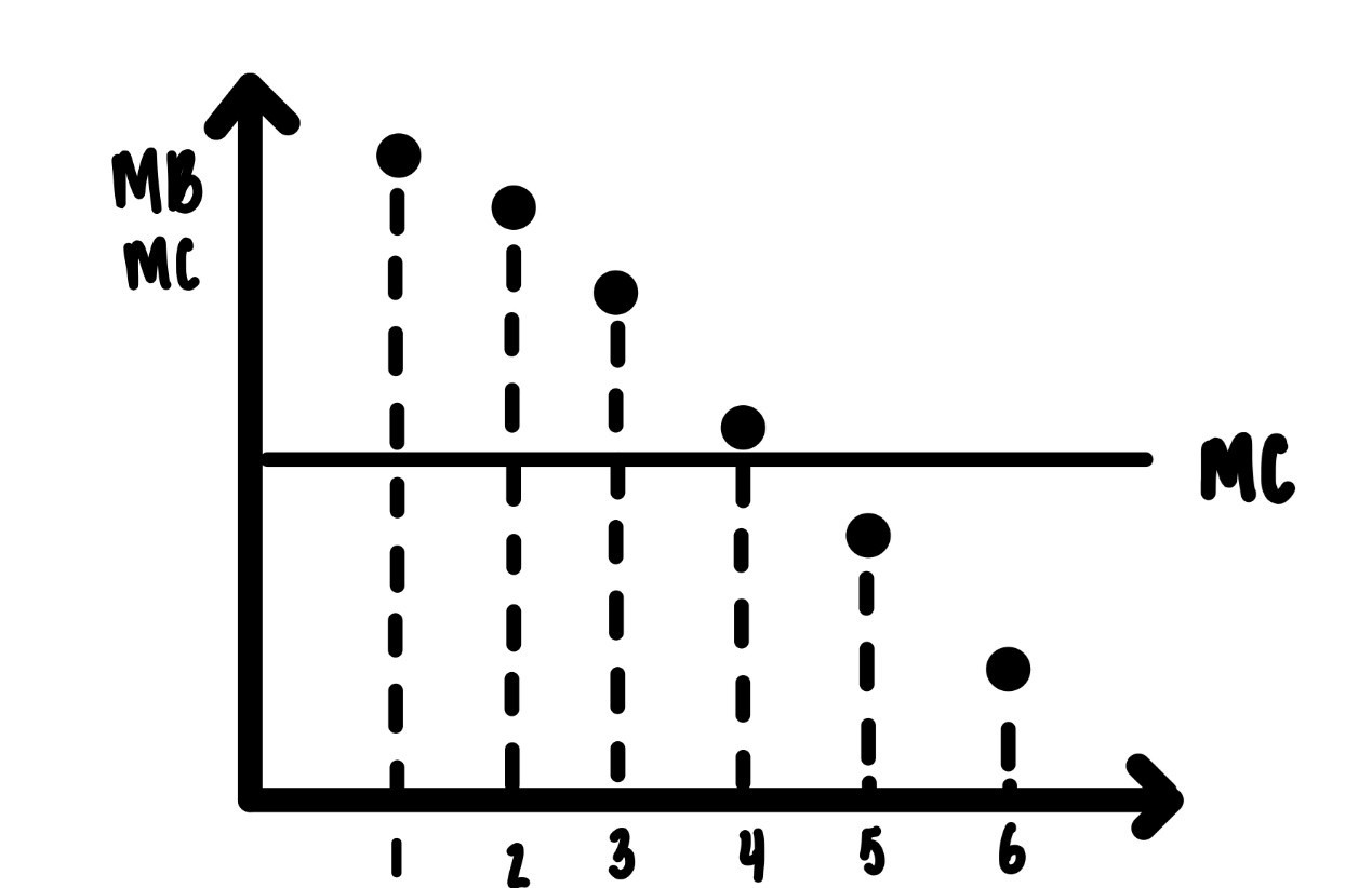
Figure 5.1: Drinking lemonade on a hot Saturday afternoon after you cut the grass.
The rational choice for lemonade consumption was exactly at the intersection of marginal benefit from the lemonade and the marginal cost of lemonade, which is, of course, the price of lemonade. This is exactly the punchline from this figure in our chapter on Rational Choice.
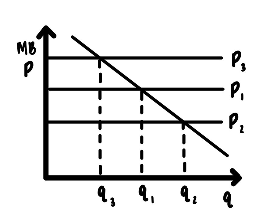
Figure 5.2: Demand for Lemonade
In Figure 5.2, here in this chapter, we show how that one consumer’s, Joe’s, rational choice of lemonade consumption changes with the price of lemonade. As the price of lemonade increases, it is rational to consume less lemonade. As the price of lemonade decreases, it is rational to consume more lemonade. In Figure 5.2 as the price of lemonade varies from \(p_1\) to \(p_2\) to \(p_3\), the rational choice of lemonade consumption varies from \(q_1\) to \(q_2\) to \(q_3\).
We can now state:
The Law of Demand: When the price of a good increases (decreases), the quantity demanded decreases (increases).
As the price varies, Figure 5.2 tells us exactly how the rational choice of lemonade consumption varies. And this rational choice of lemonade consumption is determined by the marginal benefit derived from lemonade consumption. As the price of lemonade varies from a very low value to a very high value, we sweep out the entire marginal benefit curve. This allows us to say that:
The marginal benefit curve IS the demand curve.
Or reversed, the demand curve of a product or service is the marginal benefit curve from that product or service.
Demand is the entire marginal benefit curve. Demand has to be distinguished from the quantity demanded. The quantity demanded is just one point on the demand curve. That is how much consumption is rationally chosen at a given price. Demand is the entire curve. We will always have to make this distinction.
What does demand represent? Demand represents the marginal benefit a consumer derives from a particular good. It is purely idiosyncratic. Jack’s demand for lemonade will be different from Joe’s and Joe’s demand will be different from Jill’s. That is what it is, and we will not quibble at all about what these preferences are and why they might differ.
Jack’s demand for lemonade can, of course, change over time. It will be higher on a hot summer day than on a cold November day. It will be higher in the afternoon than in the morning. Over longer periods, Jack’s preferences might also slowly shift away from lemonade, sweet and sugary, to low calorie iced tea or even water.
5.2.1 Individual to Market Demand
The analysis above involved demand from an individual consumer. How do we get from individual demand to market demand?
Easy. Just add up the individual demands. How this is done is illustrated in Figure 5.3 below for the simplest possible case of two consumers, called Joe and Mary. Joe’s demand is in panel a, Mary’s demand is in panel b.
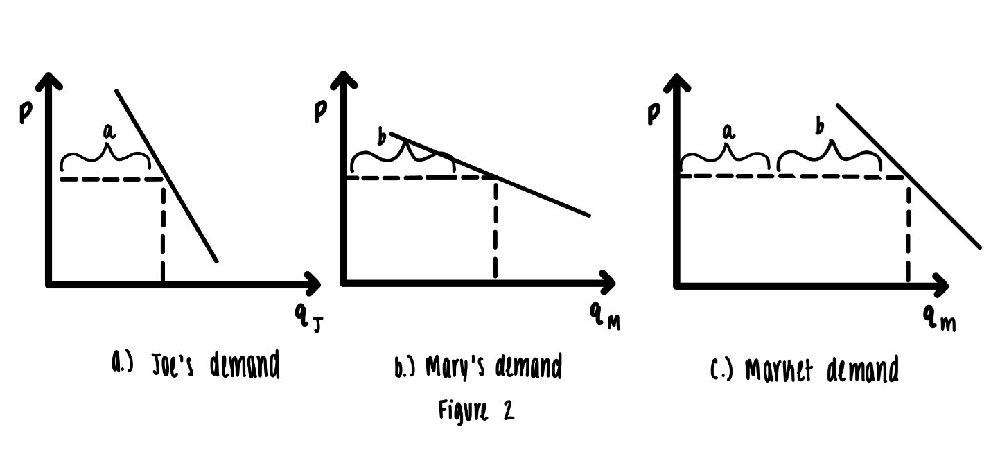
Figure 5.3: Market Demand
Both Joe and Mary face the same price. If the price is \(p_1\), then Joe’s quantity demanded is indicated by the distance “\(a\)” and Mary’s quantity demanded is indicated by the distance “\(b\)”. In panel c, these to distances are added together to get market quantity demanded to be “\(a+b\)”. We can do this at any price, not just at \(p_1\), to obtain the entire market demand function as in panel c.
This can be done for any product and for any set of consumers.
5.2.2 Alternate View of Demand
There are many products or services that are not really divisible. Either you buy them, or you don’t. Examples include large ticket items: a car, a washing machine, jet skis, or your dream vacation to Bora Bora or Glacier National Park.
Our typical view of demand is: At a particular price, how much stuff is sold? Here we go from the vertical axis, the price axis, over to demand and down to the horizontal axis, the quantity axis, and read off the quantity demanded.
We can turn this around and ask: For a particular good or service, what is the maximum amount a customer is willing to pay? Here we go from the horizontal axis, the quantity axis, up to demand and over the vertical axis, the price axis, to read off the maximum willingness to pay.
This maximum willingness to pay is sometimes called the reservation price. The reservation price is also that price which leaves the consumer just indifferent between buying or not buying.
Then, we can line up all the potential consumers in order of their reservation price, with the highest reservation prices on the left and the lowest reservation prices on the right. And, surprise, surprise, we get a downward sloping demand curve.
5.3 Elasticity
In the previous section we have established the Law of Demand, that demand is downward sloping, that an increase in the price causes a decrease in the quantity demanded. All of these statements say the same thing.
Here we will think about the slope of the demand function. Notice in Figure 5.3, Joe’s demand is a lot steeper than Mary’s demand. What determines when a demand is steep or flat? The slope of the demand function will indicate how responsive consumers are to changes in the price. This is crucial information to have when a firm sets prices of products. Total revenue will depend upon this responsiveness.
Total revenue is always price time quantity. If p is the price and q is the quantity sold by a firm, the total revenue is given by
\[TR = p \times q(p)\]
There we expressly show that the quantity sold typically depends on the price: the demand function is downward sloping. The price going up is a good thing for revenue. But then, almost invariably, the quantity goes down. This is bad for revenue. One effect is good, the other effect is bad.
Which is bigger?
That is exactly where the concept of elasticity comes in. It is easy to see that if the price goes up say 10% and the quantity goes down by 20%, the bad outweighs the good and revenue will go down.
The moral of this story is:
Know thine elasticities!
We will use the concept of an elasticity, which we denote shorthand as \(\epsilon\). Here the price elasticity is defined as
\[\epsilon=\frac{\text{percentage in quantity demanded}}{\text{percentage change in price}}\]
This concept is relatively easily illustrated with a few examples.
- If the price changes by 10% and the elasticity is 0.6, then the quantity demanded changes by 6%.
- If the price changes by 10% and the quantity demanded changes by 7%, then the elasticity of demand is 0.7.
- If we know that the elasticity of demand is 0.5 and we see that that quantity demanded has changed by 15%, then we can infer that the price has changed by 30%.
- If the price elasticity is bigger than one, a price increase will cause revenue to go down.
- If the price elasticity is less than one, a price increase will cause revenue to go up.
All of this involves very basic math. In the expression for the elasticity, there are three variables. If you know two of these, you can solve for the third. No magic required.
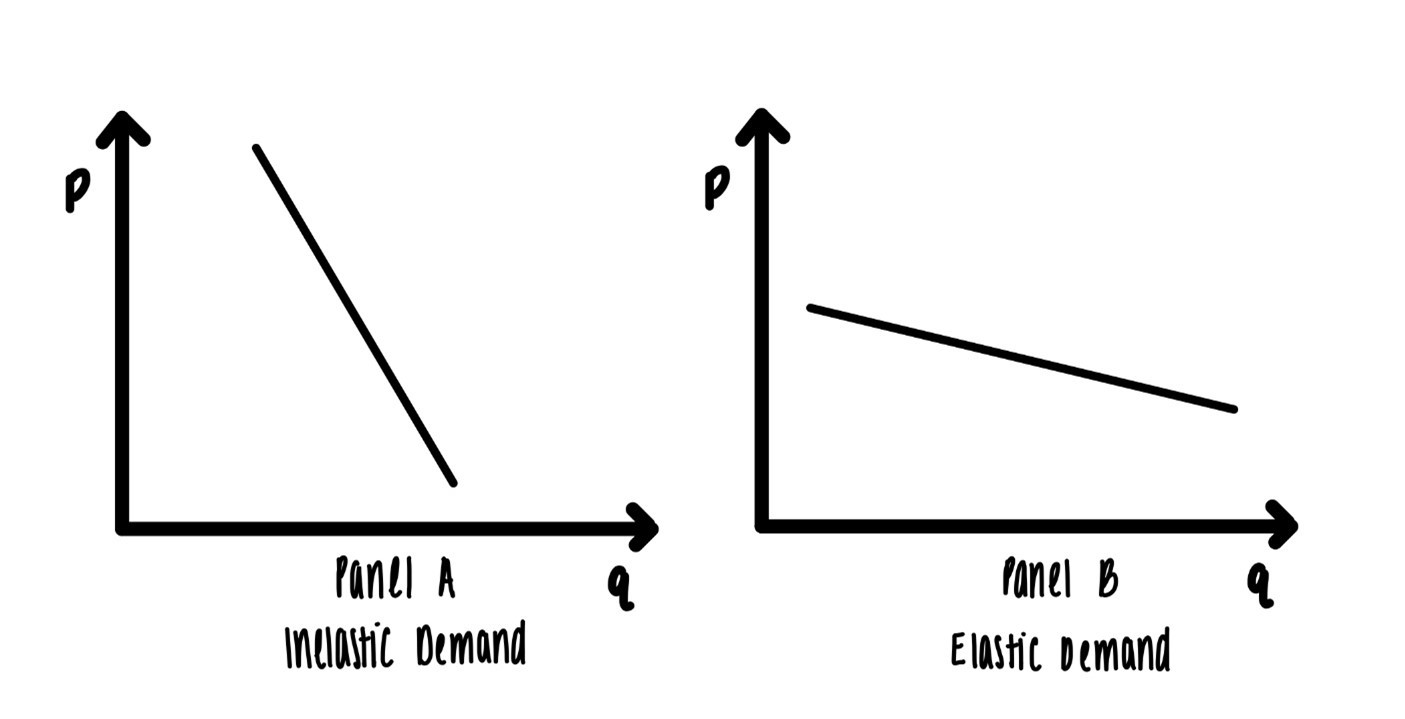
Figure 5.4: Differences in Elasticities
When the elasticity is low, the demand curve will be very steep as in panel a in Figure 5.4 . When the elasticity is high, the demand curve will be very flat as in panel b. We will speak of elastic demand when \(\epsilon\) is high and inelastic demand when \(\epsilon\) is low.
A few remarks:
In the equation/definition of the elasticity above, the elasticity is negative: When the price changes, the quantity demanded goes in the opposite direction. Hence \(\epsilon\) in the above equation is negative. In what follows we will always take the absolute value of ϵ to indicate the elasticity. The elasticity will always be a positive number.
The elasticity of demand is not an immutable law. It will vary from product to product. It will vary from consumer to consumer. Even, for individual consumers, the elasticity can vary, depending on the price. All we have are estimates of these elasticities.
The time horizon matters. When prices change, consumers often adjust. The more time that is available for the adjustment, the larger the adjustment can be. In other words: the long-run elasticities will be larger than the short-run elasticities.
Now suppose that your favorite soft drink is FSSW, Frizzy Sudsy Sugary Water and imagine that your favorite breakfast cereal is CCSB, Chocolate Covered Sugar Bombs, or is it SCCB, Sugar Covered Chocolate Bombs. Walking down the aisles in your favorite grocery store convinces you, see also Figure 5.5, that there are lots and lots of substitutes for FSSW and for CCSB.

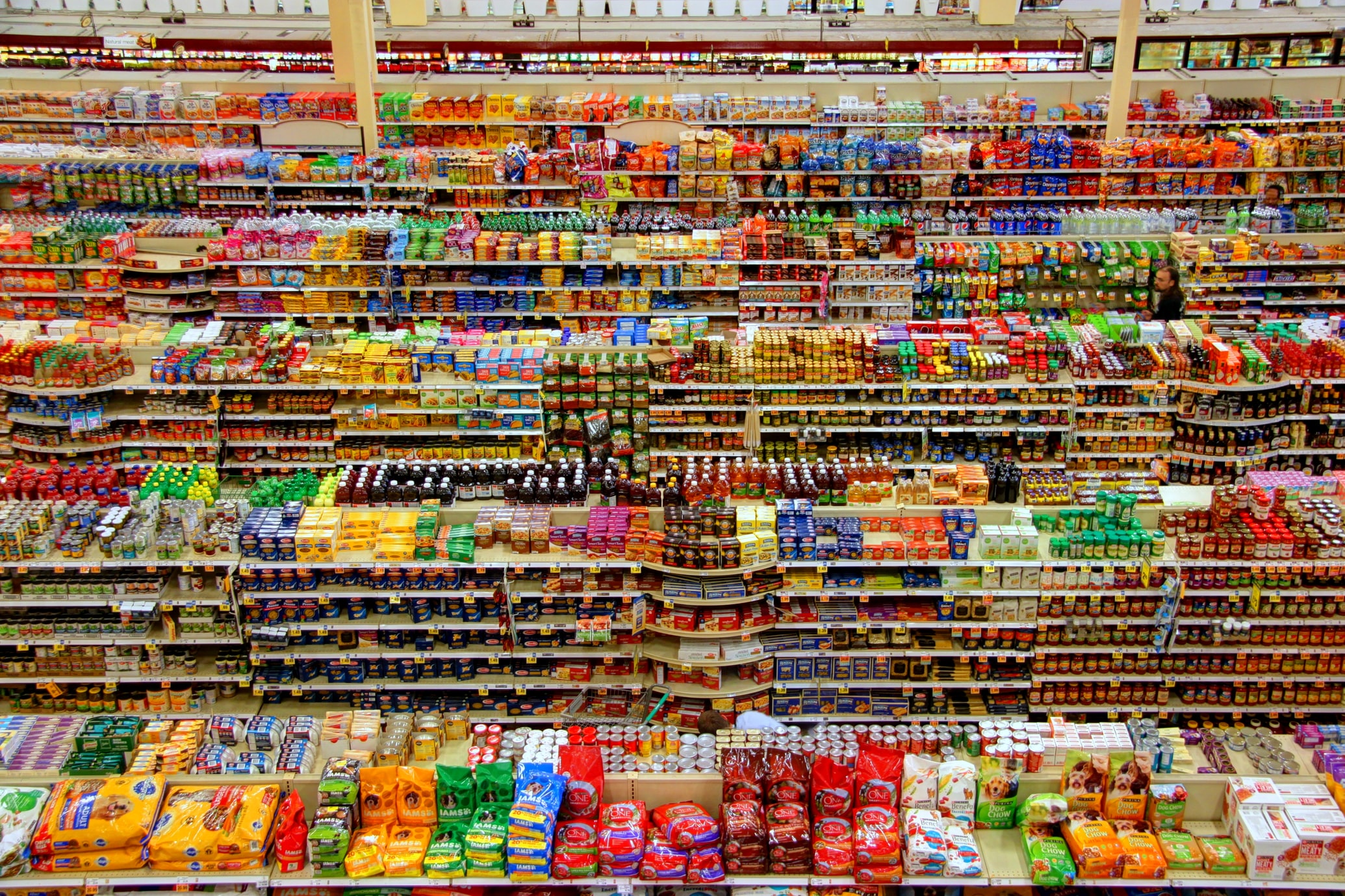
Figure 5.5: Substitutes galore. Images sourced from unsplash.
As there are tons of substitutes a small increase in the price, may induce many consumers to switch to one of the many available substitutes. In this case we would expect the demand for the product to be very elastic.
On the other hand, there are some products that have few, if any, substitutes. Two of such products are shown in Figure 5.6: coffee and toothpaste, not the particular brands, but coffee and toothpaste.


Figure 5.6: Images sourced from unsplash.
Some people would argue that there are decent substitutes available for coffee, like black tea or caffeinated soft drinks. But what do they know? For many of us, neither tea nor soft drinks are anywhere near to being decent substitutes for coffee. So, we would expect the demand for coffee to be relatively inelastic.
The same for toothpaste. There are no substitutes for toothpaste. Even if the price of toothpaste were to double or triple, I would not brush my teeth any less. Most of us would not. Again, this points to inelastic demand.
We are not talking about particular brands of coffee or particular brands of toothpaste, but about coffee in general and toothpaste in general. There is one more aspect of toothpaste that especially helps explain why we would expect demand to be inelastic: It occupies a very small part of most of our budgets. Even a doubling of price will have a relatively small impact on our purchasing power, and consequently, we will not make many, if any, adjustments in our consumption.
5.4 Substitutes
There are many goods out there that have very similar characteristics and serve very similar purposes. Figure 5.5 shows few of these cases: different soft drinks and different breakfast cereals. But there are lots of other examples. For a beach vacation, any stretch of beach between Florida and North Carolina is a good substitute for other such stretches of beach. To get my hair cut in Bloomington, there are lots and lots of suitable establishments. There are many insurance companies that would like to get my and your premium money. The list goes on and on.
It stands to reason that when we are talking about two goods that are substitutes for each other, changes in one market have an impact in the other market.
If the price of Nicaraguan coffee rises, I am very tempted to switch to Guatemalan coffee or any other of other available coffees. This would be true at any price for Guatemalan coffee. The price increase of Nicaraguan coffee results in an increase in the demand of Guatemalan coffee. In response to an increase in the price of Nicaraguan coffee, the entire demand for Guatemalan coffee increases, not just the quantity demanded. The entire demand curve shifts to the right.
In general: The demand curve shifts to the right (left), when the price of a substitute good increases (decreases). The rightward shift in demand following an increase in the price of a substitute is illustrated in Figure 5.7.
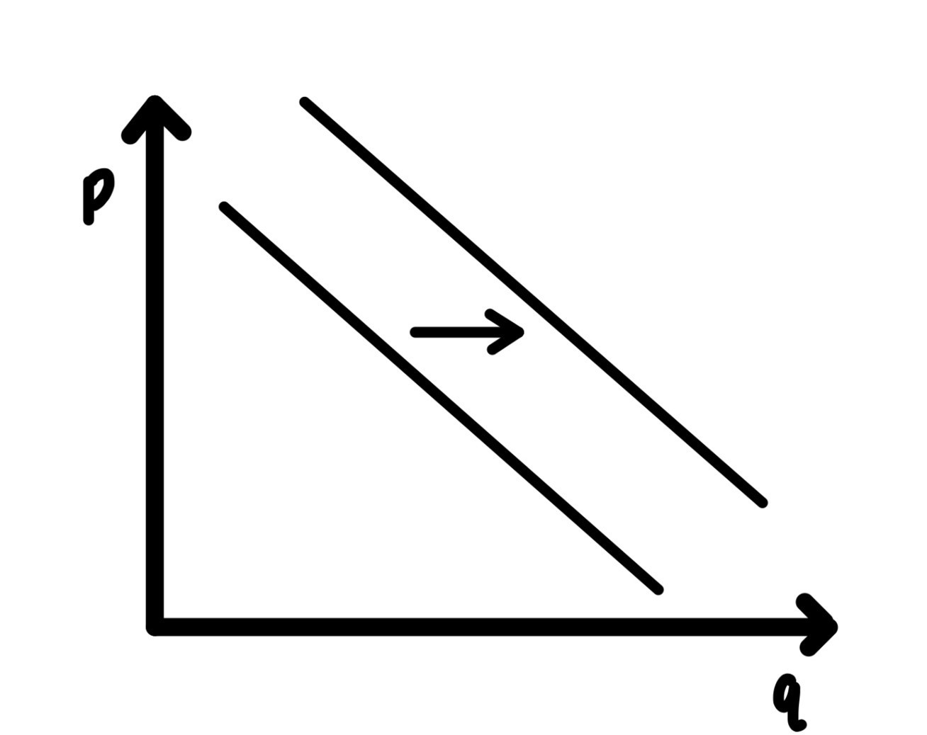
Figure 5.7: Increase in price of a substitute
Durable goods present a special case of substitutes. Durable goods are simply goods that last, perhaps even a long time. Examples include:
Cars
Kitchen table
Entertainment center
Cell phone
Fancy dress and even the non-fancy dress
Yacht
Washing machine
Road or other bike
Bedsheets and linens
And on and on.
Why are durable goods examples of substitutes? A car today is a substitute for a car next year, or a car next year is a substitute for a car today. Of course, the car next year is not a perfect substitute for the car today. We of course would prefer to have the car today, rather than waiting for the car till next year. But sometimes good things are worth waiting for. Many of us are often waiting to purchase such goods for a time when there are good deals available, for a time when prices are low. Just ask your parents, perhaps your mom, about Presidents’ Day sales for linens.
This just says that the durable good available at two different times is really two different goods that have varying degrees of substitutability. The closer the availability dates, the closer the degree of substitutability.
5.4.1 Deadly Demand
Covid can kill you in surprising ways38
We start with some sobering observations in the Figure 5.8 below. Mortality rates from narcotics overdoses, alcohol, and psychotropic drugs have been steady rising over the last decade. What we are interested here are the spikes, the large deviations from the trend, that we observe in the years 2020 and 2021.
Why was there spike, an increase in the mortality rates in the Covid years?
Could any of the Covid policies be connected to these spikes?

Figure 5.8: From Figure 2 of LETHAL UNEMPLOYMENT BONUSES? SUBSTITUTION AND INCOME EFFECTS ON SUBSTANCE ABUSE, 2020-21 by Casey B. Mulligan
We will use the simple notions of demand, supply, the elasticities of supply and demand, and shifts in supply and demand to try to make sense of these observations.
We will start with the market for alcohol. It is well known that alcohol in bars and restaurants is much more expensive than alcohol consumed at home. This price ratio has been estimated to be about 3, i.e., alcohol in bars is 3 times more expensive than alcohol consumed at home.
During the pandemic, the opportunities to consume alcohol in bars or restaurants declined, in some cases practically to nothing. Some of this was caused by the government shutting down various establishments, some was caused by some establishments closing on their own, and some of this was that going out was just not a good idea.
As the opportunities to consume expensive alcohol disappear, there will be two changes:
- An increase in the demand for alcohol consumed at home.
- A massive slide down along the demand curve since alcohol consumed at home costs only one third of alcohol consumed so that there is a massive drop in the price. The law of demand will kick in massively.
So much for theory! How big can these effects be? Mulligan uses an estimate of the price elasticity of the demand for alcohol of around 0.85 in absolute value to conclude that such a large drop in the price must be accommodated by a very large increase in the quantity of alcohol consumed. A large increase in alcohol consumed leads to the spike in alcohol-related deaths.
The spike in alcohol related deaths is explained.
But.
But, hold it.
Excessive alcohol consumption leads to liver disease and failure of the liver. Slowly and gradually.
Slowly and gradually.
There is no way the excessive alcohol consumption in 2020 can lead to alcohol related deaths spiking in the same year.
Case closed.
No! No! No!
There are a variety of alcohol related causes of death:
- Pseudo-Cushing syndrome
- Degeneration of nervous system due to alcohol
- Alcoholic polyneuropathy
- Alcoholic myopathy
- Alcoholic cardiomyopathy = Alcoholic gastritis
And a few more. (As an aside, it can be really useful to know human biology!)
These are the kinds of conditions associated with the mortality data and the spike in alcohol related deaths in Figure 5.8 above.
5.5 Complements
Some of the goods we buy have synergies with one good enhancing the usefulness or enjoyment of the other good. We call these kinds of good complements. Examples abound.
Skis and ski lift tickets.
Bicycle and helmet.
An econ and a stats class.
Haircut and beard trim.
Burger and beer.
Washer and drier.
Computer and printer.
And so on and so an.
If the price of computers rises, by the law of demand, fewer computers will be purchased. Since printers are complements to computers, fewer printers will be sold as well. In other words, as the price of computers rises, the demand curve for printers shifts to the left.
In general: The demand for a good shift to the left (right), as the price of a complement good rises (falls).
This is illustrated in Figure 5.9 for the case of a price increase of a complement.
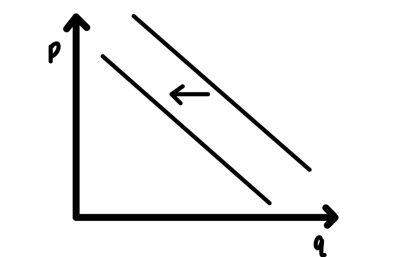
Figure 5.9: Increase in price of a complement
5.6 Substitutes Complements in Unexpected Places
Many disasters strike in this country: tornadoes, hurricanes, wildfires, floods, mass shootings, earthquakes, etc., etc., etc. High profile politicians and private citizens invariably offer their condolences in words like:
“You are in our thoughts and prayers.”
“You are in my thoughts.”
“You are in my prayers.”
One could easily argue that what matters most to victims in such cases is actual help. Having homes rebuilt and having financial resources to rebuild their lives.
Thoughts, prayers, actual assistance? What is the relationship between these three? Are they substitutes or complements? How could we find out?
Well, you set up a field experiment. Right after a hurricane you take a sample of 472 religious Christians and 487 atheists or agnostics. Participants in the field experiment are either given the “thoughts experiment”, the atheists or agnostics, or the “prayer experiment”, the religious Christians. In either group, participants were given an opportunity to offer either thoughts or prayers, depending on which group they belonged to, either by itself or in conjunction with an actual monetary donation to the hurricane victims.
Results39:
- The gesture, thoughts or prayer, depending on the group, are popular ways of showing support for the victims.
- There is substantial “crowding out”: The share of participants not making any donations increased to 59% in the “thoughts” experiment, the atheists/agnostics and to 71% in the “prayers” experiment for the religious Christians, from a common baseline of 33% for both groups. Greater crowding out for the religious Christians.
- Relative to baseline, the amounts donated changed differently in the two groups as well. Participants in the “thoughts” group contributed 48% less relative to base; the participants in the “prayer” group contributed 60% less relative to base.
Conclusion: Both “thoughts” and “prayers” seem to be substitutes for action/donations. Perhaps next time someone offers “thoughts and prayers”, you might think about the actual value of those gestures. Are they hollow?
How large are these effects? The authors claim that for the entire country, this effect may amount to hundreds of millions of dollars. Imagine what a Red Cross official might say of you ask whether a couple hundred million dollars is a big or a small number.
The findings here fit in and are consistent with the literature on “moral licensing”. Other examples of moral licensing are:
- Some people are more likely to act in prejudiced ways after expressing politically correct views.
- Some people are more willing to cheat and lie after buying a green product.
It seems there is, in some peoples mind an ethical budget, a good behavior budget. If one type of good behavior goes up, the other one must go down. Now there is a challenge for all ethics teachers.
5.7 Normal and Inferior Goods
Most goods are normal, that is why we call them that.
A normal good has the following property: as income increases, demand increases. The entire demand curve shifts to the right if income increases. This is illustrated in panel a of Figure 8. There are also inferior goods. An inferior good has the following property: as income increases, demand falls, the entire demand function shifts left. This is illustrated in panel b of Figure 5.10.
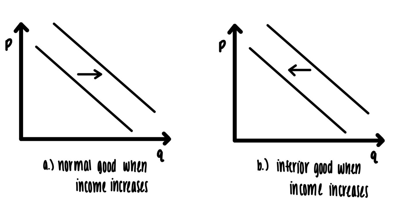
Figure 5.10: Price increases
5.7.1 Product Quality
The demand function of course depends upon the quality of the product or service. High quality stuff has high demand, low quality stuff has low demand. This simply works because demand IS marginal benefit. High quality stuff is highly satisfying and has high marginal benefit and this high demand, low quality stuff not so much. Demand for IU basketball games would be higher if the quality of the product were higher. Of course, sometimes it is just the perception of quality, not the real quality that matters.
So, what is quality? In some cases, it is easy to determine quality. Not so much in others.
In the paper below https://www.cesifo.org/en/publikationen/2021/working-paper/demand-fact-checking the authors take on this question for the case of “news”. You might think that most people would consider accurate news higher quality and thus have higher demand for more accurate news.
If that is your belief, you would be wrong.
The authors set up an experiment with a treatment group and a control group. The treatment group gets an offer for a newsletter with fact checking and the control group gets the same offer of a newsletter, but without the promise of the fact check. One would think that fact checking will make for more accurate, and thus better, news and hence higher demand.
To simplify the problem a bit, the researchers pick one side of the ideological spectrum. They could have picked Democrats or Republicans. They picked Democrats. The newsletter then covered topics associated with The American Rescue Plan Act of 2021, the Biden Rescue plan.
If fact checking provides more accurate news and if more accurate news is a better product, we would expect higher demand for the newsletter in the treatment group that received the fact checked newsletter.
This is not so.
There is no statistically significant difference in the demand for the two types of newsletter.
There is a statistically different assessment of the accuracy of the newsletter. But that difference does not seem to matter for demand.
What is going on? The researchers divided the recipients of the newsletters into two groups, those with stronger ideologies and those with weaker ideologies. We can think of the people with stronger ideologies as more left leaning and the one with weaker ideologies as being more centrist.
Here is the kicker: Fact checking increases the demand for the newsletter for people with weaker ideologies. But fact checking DECREASES the demand for the newsletters for people with strong ideologies. The two effects cancel each other out.
Conclusion: Some people are not so much interested in facts as in confirming their own preconceived notions.
5.7.2 Uncertainty
The typical textbook does not list uncertainty as a factor that can shift demand. It should. Consider the demand for big ticket items, durable goods like cars, boats, big entertainment centers, etc. Or even big tickets items that are not durable, like your super fancy vacation on Bora Bora.
Consider Jack and Jackie who are identical in all aspects, except that one faces a certain income stream and the other an uncertain income stream. To fix ideas, assume that his income is fixed at a particular level and this is known with certainty. The income growth for Jackie is uncertain. Here income is up next year by \(\$1000\) with probability 0.9 and it is down next year by \(\$9,000\) with probability 0.1. Both Jack and Jackie have the same expected income, but hers is more uncertain. If she gets the bad draw, she might not be able to make rent/mortgage payments.
Which of the two will have higher demand for big ticket durables?
Most of us will guess that Jack has higher demand for such big-ticket items. If Jackie is at all risk averse, she might forego the purchase of such items in order to ensure that she can make the rent/mortgage payment.
Is this just ivory tower theorizing? The answer is a definite NO.
The paper here shows that macroeconomic uncertainty during COVID-19 did indeed reduce demand for certain goods.
The analysis is not exactly straightforward.
See, you can’t just ask people: How uncertain do you expect future income to be? And then correlate that with some measure of their consumption. This will not work because there could be some other hidden factor that cause both uncertainty and consumption levels. We don’t want to estimate the effect of that factor, we want to estimate how uncertainly, and only uncertainty, influences consumption.
So, we have to work harder. We start with people’s perception of income uncertainty. Then we split households into several groups. Some households receive information about what experts think income uncertainty will be, and other households do not receive such information. The assignment into these groups is random, so we have a treatment group and a control group.
Providing this information, or not, may have an influence on households’ beliefs on future income uncertainty. It may or may not; one has to check. It turns out it does. This change in beliefs about income uncertainty will be exogenous.
Now we are in business. We can estimate how that exogenous change in beliefs influences consumption. The above paper finds:
A one standard deviation increase in exogenous beliefs about future income uncertainty reduces consumption of non-durable goods by almost 5 percentage points, i.e., increasing income uncertainty shifts demand to the left, even for non-durables. Similar results are obtained for big ticket items like fancy vacation packages and expensive jewelry.
Why is this paper important?
Natural disasters by their very nature increase uncertainty and Covid-19 is no exception. Covid-19 generated the sharpest drop into a deep recession in many countries. Much of the policy discussion now, Spring of 2021, focuses on the economic costs of the shutdown. The shutdown has certainly decreased consumption, but it is wrong to claim the entire drop in consumption is due to the shutdown. The above paper shows that a sizeable drop in consumption is due to just increased uncertainty due to the natural disaster. So much of that is independent of policy.
Questions:
- Is it moral licensing to make a significant contribution to Green Peace or similar organizations and then book a 4-week vacation on Bora Bora?
- Is it moral licensing to induce fast food establishments to give up plastic drinking straws, but then drive an SUV?
- What are the relative prices of these actions?
5.8 Glossary of Terms
Complements: Two or more goods are called complements if consumption of one good enhances the marginal benefit of the other good.
Demand: see Individual demand, Market demand
Elasticity of Demand: The absolute value of (the percentage change in the quantity demanded/the percentage change in the price).
Endogenous variable: a variable that is determined inside the model
Exogenous variable: a variable that is determined outside the model.
Individual Demand: Demand is the entire collection of points where the marginal benefit of a good or service is equal to the price, for all possible prices and for one individual. This is the entire curve.
Inferior Good: A good is called inferior if an increase in income shifts demand to the left.
Market Demand: Market demand is obtained by horizontally adding the individual demands of all consumers in the market at a particular price and then repeating the procedure for all possible prices. This traces out the entire curve.
Normal Good: A good is called normal if an increase in income shifts demand to the right.
Quantity Demanded: The quantity demanded at a price is the amount of the good or service where the marginal benefit of the good or service is equal to the price of good or service. This is the amount of the good or service that a rational consumer would consume at that price. This is one point on the demand curve.
Reservation Price: The reservation price is the maximum amount a customer is willing to pay for a product. It is also the price where the customer is just indifferent between purchasing the good or not.
Substitutes: Two or more goods are called substitutes if they have similar characteristics and/or serve similar purposes.
5.9 Practice Questions
5.9.1 Discussion
- Imagine that the price of gasoline doubles starting next month and is expected to stay that high in the foreseeable future. List all the adjustments consumers could make within a week, within a month, within a year, and withing a 5 to 10-year horizon. What would you expect the price elasticities of demand for gasoline to be in any of these horizons?
- Which of the following goods are normal, which are inferior? Socks, restaurant meals, polyester pants, IU, potatoes, fresh strawberries, bus tickets, Broadway shows, lard sandwiches? Does it matter whether we are considering the suburbs of Chicago or the poorest rural counties in Indiana?
- Without reading the article below, since washers and dryers are complements what would you expect to happen to the demand for dryers after a tariff was imposed on washing machines? Now, read the article below. https://news.uchicago.edu/story/what-washing-machines-can-teach-us-about-cost-tariffs What DID happen to the price of dryers after there was a tariff on washing machines? How can you explain that?
5.9.2 Multiple Choice
-
According to the law of demand, an increase in the price of cauliflower
A. Increases the demand for cauliflower
B. Decreases the demand for cauliflower
C. Increases the quantity demanded of cauliflower
D. Decreases the quantity demanded of cauliflower -
As the marginal benefit curve for a product shifts to the right,
A. The demand curve shifts to the left
B. The demand curve shifts to the right
C. The marginal cost increases
D. The marginal cost decreases -
Jack and Jill both love to eat burgers. Jill is more openminded than Jack and would consider eating non-meat-based burgers. Jack would never consider non-meat-based burgers. Based on this information
A. Jack’s demand for burgers is higher than Jill’s
B. Jack’s demand for burgers is lower than Jill’s
C. Jack’s demand for burgers is more elastic than Jill’s
D. Jack’s demand for burger’s is less elastic than Jill’s -
The Simpson’s price elasticity for gasoline in the short run is 0.1 in absolute value. The price of gasoline rises by 20%. Then their demand
A. Rises by 2%
B. Falls by 2%
C. Falls by 0.2%
D. None of the above -
The Simpson’s price elasticity for mouthwash is 0.01 in absolute value. The price of mouthwash rises by 50%. Then quantity demanded of mouthwash
A. Rises by 5%
B. Falls by 5%
C. Rises by 0.5%
D. Falls by 0.5% -
Mouthwash and toothpaste are complements. The price of toothpaste rises by 25%. Then
A. The quantity of toothpaste demanded falls
B. The demand for mouthwash rises
C. The demand for mouthwash falls
D. a. and c. -
Shinywhite and Whityshine are two toothpastes. The price of Shinywhite rises by 35%. Then
A. The quantity demanded of Shinywhite rises
B. The demand for Whityshine falls
C. The demand for Whityshine rises
D. a. and c. -
Jack and Jill are social scientists. Their interests are the driving habits of Americans. Jack studies the elasticity of the demand for gasoline by taking measurements of driving behavior one month after substantial gasoline price changes. Jill takes similar measurements, but two years after such changes in prices. Then, in absolute value,
A. Jack’s estimate of the elasticity will be the same as Jill’s
B. Jack’s estimate of the elasticity will be higher than Jill’s
C. Jack’s estimate of the elasticity will be lower than Jill’s
D. Jack’s estimate of the elasticity by at least twice as high as Jill’s -
The estimates of the elasticity of demand tend to increase if longer time horizons are considered because
A. Supply is elastic
B. Supply is inelastic
C. Over time, households will find themselves more and more locked in
D. Over time, household will tend to find more ways to adjust their behavior -
Potatoes are considered an inferior good. As a community gets richer over time, we would expect
A. The demand for potatoes to increase
B. The demand for potatoes to decrease
C. The demand for potatoes to become more elastic
D. The demand for potatoes to become less elastic -
As communities get richer and richer the variety of fresh fruits offered in their grocery stores increases. (If you don’t believe that, you may want to ask your grandparents.) Then we would expect over time
A. The demand for oranges to become more elastic
B. The demand for oranges to become less elastic
C. The demand for oranges to increase
D. All of the above -
There are two goods, X and Y. We observe that as the price of X rises the demand for Y falls. We may conclude that
A. Y is a normal good
B. Y is an inferior good
C. X and Y are substitutes
D. X and Y are complements -
The availability of Covid-19 vaccinations and the widespread use of such vaccines has drastically reduced the risk of getting infected in a restaurant. We would expect this declining risk of getting infected to
A. Decrease the demand for restaurant meals
B. Increase the demand for restaurant meals
C. Make the demand for restaurant meals less price elastic
D. All of the above -
The price elasticity for movie tickets is 0.8. Then a price increase in movie tickets leads to
A. In increase in demand
B. A decrease in demand
C. An increase in revenue
D. A decrease in revenue -
The price elasticity for movie tickets is 1.2. Then an increase in the price of movie tickets leads to
A. An increase in the quantity of movie tickets demanded
B. An increase in revenue
C. A decrease in revenue
D. a. and c -
The quantity of soft drinks demanded is where
A. The marginal benefit from soft drinks is bigger than the price
B. The marginal benefit from soft drinks is smaller than the price
C. The marginal benefit from soft drinks is equal to the price
D. None of the above -
Imagine that IU cuts its undergraduate enrollment drastically from 30,000 undergraduates to 10,000, thereby bringing about a substantial reduction in hiring of faculty and staff. This reduction in faculty and staff size will
A. Decrease the demand for running shoes in Bloomington
B. Increase the demand for running shoes in Bloomington
C. Make the demand for running shoes in Bloomington less elastic
D. Make the demand for running shoes in Bloomington more elastic -
Jill likes women’s college basketball. Her reservation price for a typical single IU game is $10. In two weeks, the nation’s top ranked team comes to town. For that game we would expect
A. Jill’s reservation price to be above $10
B. Jill’s reservation price to be below $10
C. Jill’s reservation price to stay at $10
D. Jill’s reservation price to double -
IU and PU are competing for students. There is plenty of relevant information available about these to universities so that students can make ration choices and determine their reservation prices to attend each one of these institutions. While the students are deliberating their choices, a new ranking shows that the job placement rates for PU students has skyrocketed. This new information will
A. Increase the reservation price to attend IU
B. Decrease the reservation price to attend IU
C. Leave the reservation price to attend IU unchanged
D. Double the reservation price to attend IU -
Which one of the following has the highest, in absolute value, elasticity of demand?
A. Coffee
B. Organic coffee
C. Fair trade coffee
D. Organic fair-trade coffee