11 Oligopoly

In this chapter we will learn:

• Understand the basic application of game theory to markets with large firms
• Understand how the Cournot equilibrium is constructed
• Describe the properties of the Cournot equilibrium
• Describe the properties of the Bertrand equilibrium
• Understand simple game theoretic models of product differentiation

11.1 Motivation

American industry is highly concentrated, now more than 50 years ago. You might get the impression by walking into your favorite store that there is lots and lots of choice and tons and tons of competition. It does not matter what store you walk into to get that impression: a grocery store, a clothing store, liquor store, a home improvement store, etc. You will be blown away by the plethora of choices. The number of breakfast cereals, the varieties of cat food, the number of different kinds of bedsheet and window blinds is staggering.

But this does not spell competition.

Figure 11.1 below (Eeckhout 2021) shows some illustrative examples of how highly concentrated many markets are.

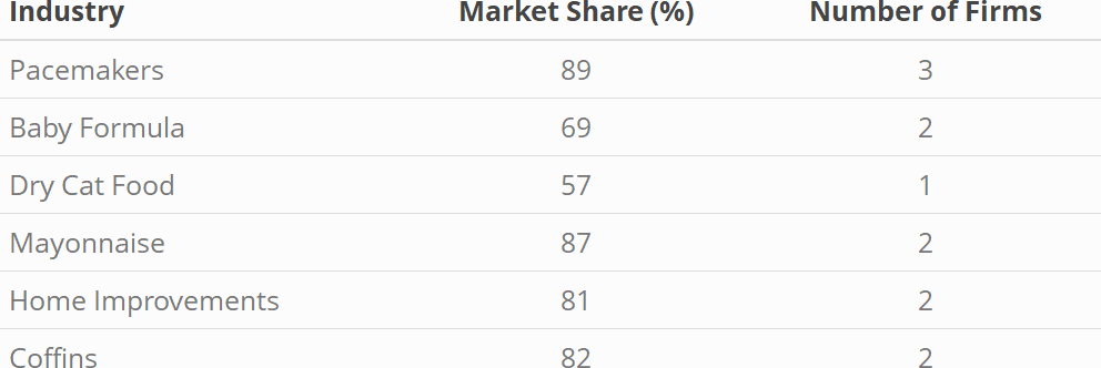
Figure 11.1: Market Concentrations

We have to understand how markets with such large concentrations work.

• How do individual firms in such markets behave?
• What are the equilibria in such markets like?
• What are other economic repercussions of such behavior/equilibria?

11.2 Cournot Equilibrium

In this section we study the simplest case of an oligopoly, a duopoly, that is an oligopoly with two firms. These two firms produce an identical product. The cases of heterogeneous products will be considered later.

As a reference point, we start with monopoly pricing, so this is a bit of a review.

Assume the demand is given by (Recall, \(Q\) denotes market quantity, but we are in the case of monopoly, ie one firm, so \(Q=q_1\), or in words, firm quantity is market quantity.)

\[P = 20 – Q\]

and that marginal cost is given by \(MC = 9\). The profit maximizing calculation is illustrated in Table 2 below (recall \(MB=MC\))

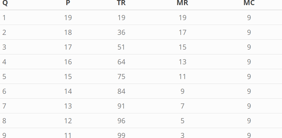
Figure 11.2: Monopoly pricing calculation

The upshot from Figure 11.2 is the profit maximizing quantity is \(Q = 6\) with corresponding price: \(P=14\) and profit \(\pi=30\)

Let’s keep these numbers in mind when we think about the duopoly. We assume exactly the same demand and the same marginal cost. Now, the decisions of one firm will depend upon the decisions of the other firm. That is since \(Q\) is market quantity and we now have more than one firm: \(Q=q_1+q_2\).

So, let’s assume that firm 1 produces 3 units. That leaves a residual demand for firm two of

\[P = 17 – Q\]

Given that residual demand we can do Firm 2’s profit maximization calculations. These are contained in Table 11.1.

Table 11.1: Firm 2s profit maximizing calculation if firm 1 sells 3 units

Q2	P	TR2	MR2	MC
1	16	16	16	9
2	15	30	14	9
3	14	42	12	9
4	13	52	10	9
5	12	60	8	9
6	11	66	6	9
7	10	70	4	9
8	9	72	2	9
9	8	72	0	9

Given these numbers, it is best for firm 2 to produce somewhere between 4 and 5 units.

But now something is wrong, does not add up. Firm 1 produces 3 units and firm 2 produces over 4? Why would there be a difference in the output of these two firms, when they are equal? They produce the same good and they have the same cost. They are equal. If they are equal, should they not produce the same amount?

And, besides: If firm produces between 4 and 5 units, how do we know that producing 3 units is in the best interest of firm 1? That is the Nash condition of best response. We certainly cannot take that for granted.

We need to check that firm 2s output is a best response to firm 1s output.

AND

We need to check that firm 1s output is a best response to firm 2s output.

We need both actions to be best responses to each other. So onward we go.

In Table 4 we illustrate firm 2s profit maximization when firm 1 is assumed to produce 5 units. Then firm 2s residual demand is \[P = 15 - Q\]

How firm 2 responds to firm 1 producing 5 units is illustrated in Table 11.2 below.

Table 11.2: Firm 2s profit maximization calculation when firm 1 sells 5 units

Q2	P	TR2	MR2	MC
1	14	14	14	9
2	13	26	12	9
3	12	36	10	9
4	11	44	8	9
5	10	50	6	9
6	9	54	4	9
7	8	56	2	9
8	7	56	0	9
9	6	54	-2	9

It is apparent from Table 11.2 that firm 2 will produce between 3 and 4 units if firm 1 produces 5 units. That means as firm 1 produces more, firm 2 responds by producing less. But we still have not found the Nash equilibrium?

But we are close!

What happens to firm 2 if firm 1 produces 4 units. See Table 11.3 If firm 1 produces 4 units, it is profit maximizing to also produce 4 units. Since the situation is totally symmetrical, we can just exchange the names of the firms. If firm 2 produces 4 units, it is profit maximizing for firm 1 to also produce 4 units.

Bingo!

Shangri La!

We have arrived at Nash equilibrium! Each firm’s action is a best response to the other firm’s actions. That is the definition of Nash equilibrium.

Table 11.3: Nash Equilibrium

Q2	P	TR2	MR2	MC
1	15	15	13	9
2	14	28	11	9
3	13	39	9	9
4	12	48	7	9
5	11	55	5	9
6	10	60	3	9
7	9	63	1	9
8	8	64	-1	9
9	7	63	-3	9

When each firm produces 4 units, total industry output is 8.

Then the price is 12.

Total industry profit is 24.

While this example is quite specific, the general conclusion from this example is:

1. As the number of firms increases from 1, a monopoly, to two, a duopoly, each individual firm produces less.
2. As the number of firms increases from 1, a monopoly, to two, a duopoly, total industry output increases.
   
3. As the number of firms increases from 1, a monopoly to two, a duopoly, the price decreases.
4. As the number of firms increases from 1, a monopoly, to two, a duopoly, the profit for each single firm decreases.
5. As the number of firms increases from 1, a monopoly, to two, a duopoly, the overall industry profit decreases.

We can actually calculate similar equilibria for any number of firms. This just takes a little math. The results that emerge from such an exercise are:

1. An increase in the number of firms implies a decrease in output by each firm.
2. An increase in the number of firms implies an increase in total industry output.
3. An increase in the number of firms implies a decrease in the price. Given 2. This is just the Law of Demand
4. An increase in the number of firms decreases the profit for each firm
5. An increase in the number of firms decreases the total industry profit.

One can actually show that as the number of firms increases and gets very large, the equilibrium gets closer and closer to the competitive equilibrium. This is true in the following sense:

• The quantity converges to the competitive equilibrium quantity, which is the efficient quantity.
• The price converges to the competitive equilibrium price.
• The profit converges to the competitive equilibrium profit, which, in the long run, is zero.

This kind of Nash equilibrium is named after Antoine Augustin Cournot and is commonly referred to as Cournot Nash equilibrium or just Cournot equilibrium. See https://en.wikipedia.org/wiki/Antoine_Augustin_Cournot

Monsieur Cournot!

11.3 Bertrand Equilibrium

In the Cournot equilibrium each firm chooses the quantity to maximize its profit, assuming that the other firms do the same. We say that

Quantity is the strategic variable.

This kind of equilibrium is not the only way to think about strategic interactions between oligopolists. There is another theory that holds that

Price is the strategic variable.

When price is the strategic variable, the nature of the equilibrium changes fundamentally. We can illustrate this easily with two firms that sell an identical product. The figure below shows profit for one of the two firms, as a function of the price charged by the other firm. That figure shows that

1. If my price is lower than yours, I will get the entire market and my profit is rising in the price.
2. If my price is equal to yours, we will split the market and my profit will be about half of what it would be if I just slightly undercut you.
3. If my price is higher than yours, my market will be zero.

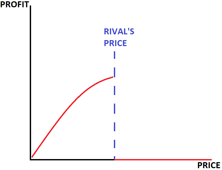
Figure 11.3: Price and Profit

That picture makes the incentive to undercut each other very clear. If my price is just a tad higher than yours, I get nothing. But if I just slightly undercut you, I get the entire pie.

So why would I not undercut you??

But the same is true for you as well.

If you charge \(\$10\), I will charge \(\$9.95\).

Then you will charge \(\$9.90\) and I will undercut you by charging \(\$9.85\).

Where will this undercutting stop?

It will go all the way down to marginal cost. Profit is eroded.

In game theory speak:

• My best response to you, whatever price you charge, is to undercut you.
• Your best response to me, whatever price I charge, is to undercut me.

This kind of an equilibrium is called a Bertrand equilibrium, after Joseph Louis Francois Bertrand.

https://en.wikipedia.org/wiki/Joseph_Bertrand

The above analysis has assumed that the product sold is homogeneous and the strong undercutting incentive is certainly due to that assumption. The figure below will show how that strong undercutting incentive will change when there is product differentiation, when the products are different.

When my product is different from yours, my cereal may have more fiber than yours, my beer may be hoppier to make the customers happier than yours, etc. etc., then I can charge a higher price that you without losing all my customers, because some of my customers will by my product because if the fiber or the hoppiness. In the figure below, my profit shrinks as my price inches above yours, but certainly not as precipitously as in the homogeneous product case.

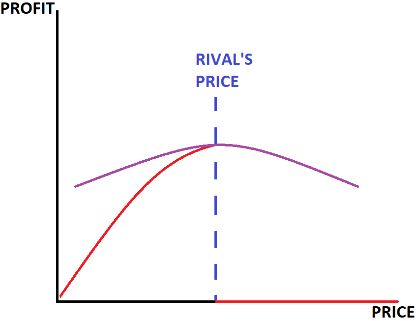
Figure 11.4: Price and Profit under slightly differentiated products

One of the lessons that might emerge from the above analysis is that it pays to be different. Offering a differentiated product will give your customers another reason, besides price, to purchase your product.

11.4 Mergers: Intro and Some Theory

We often see two independent firms combining to form one firm. These combinations of independent firms are called mergers. Two or more firms merging, of course, reduces the number of firms. In 2021 and 2022 there were about 20,000 mergers per year.

Sometime these mergers occur in waves, in periods when the number of mergers rises, to be followed by periods where fewer mergers occur. In the United States the merger waves over the last century occurred in

The 1920s

The 1960s

The early 1980s

And

The period from 1995 to 2010

There are different types of mergers.

A conglomerate merger is a combination of two firms in totally unrelated markets. A chain of nail salons merges with a bicycle factory. Imagine that!

A horizontal merger combines two firms in the same industry. Gerhard’s Pretty Decent German Bakery is combined with Jacque’s Delicious Croissants.

In a vertical merger one firm is combined with other firms that are either customers or suppliers of the firm. Gerhard’s Pretty Decent German Bakery is combined with Fritz’s Fine Flour.

There are other types of mergers, but these are the three major types we will concentrate on.

We will start with horizontal mergers. What would economic theory say about the potential consequences of mergers? These consequences could come in two categories:

1. Potential increases in efficiency
2. Potential increases in the price-marginal cost mark-up

Efficiency gains could arise for two reasons.

First: After a merger, the consolidated firm may have several plants that are of variable efficiency. Then it might be in the interest of the firm to shut down inefficient plants or at least to shift more resources to the more efficient plants. In either case we would expect marginal costs to drop. And as marginal costs drop, economic theory predicts that the price drops, the quantity sold increases and profit increases.

Second: After the merger the consolidated firm may be in a better position to exploit economies of scale. It might be the case that average variable cost is downward sloping. Then it would be profit maximizing to produce more after the merger than before.

Third: The mark-up of price over marginal cost is likely to increase. Any merger decreases the number of firms, and this potentially decreases competition. In the Cournot-Nash equilibrium the price would rise, the quantity would fall as the number of firms is reduced. At least that is the theoretical prediction.

We have to note that these are potential effects. These are predictions of some models.

Which of these effects will be realized by mergers in general or by a specific merger in particular? Which of these effects will show up in the data? That is the $64,000 question.

In order to answer that question, we have to look at data.

11.4.1 A Look at General Data

This is exactly what Blonigen and Pierce (2016) do with a comprehensive data set covering the entire US manufacturing sector from 1997 to 2007. They estimate efficiency gains, i.e., decreases in marginal costs and increases in the mark-up separately. In order to identify these effects, they use:

1. Productivity before and after the merger
2. Productivity of firms that were merged and those that were not
3. Mark-ups before and after the merger
4. Mark-ups by firms that were merged and those that were not

The findings are:

1. There are no statistically significant changes in productivity
2. There are statistically significant changes in the mark-ups. These are consistent with that theory predicts.

The increases in the mark-ups are large with 13% of the average mark-up.

Here is the authors’ conclusion:

“We find that evidence for increased average markups from M&A activity is significant and robust across a variety of specifications and strategies for constructing control groups that mitigate endogeneity concerns. In contrast, we find little evidence for plant- or firm-level productivity effects from M&A activity on average, nor for other efficiency gains often cited as possible from M&A activity, including reallocation of activity across plants or scale efficiencies in non-productive units of the firm.”

11.4.2 A Particular Merger

In 2007 a mega merger occurred in the health care sector. It involved two large hospital chains consisting of over 100 hospitals. There is a lot of data that allows extensive evaluation of the effects of this merger.

https://papers.ssrn.com/sol3/papers.cfm?abstract_id=3961070

The data in Figure 11.5 sets the scene. It allows a look at the situation of the for-profit health care market the year before the merger. The first column has data for the hospitals owned by the acquiring company, the second column has the equivalent data for the hospitals owned by the target, the to be acquired company, and the last column has a comparison to other for-profit hospitals.

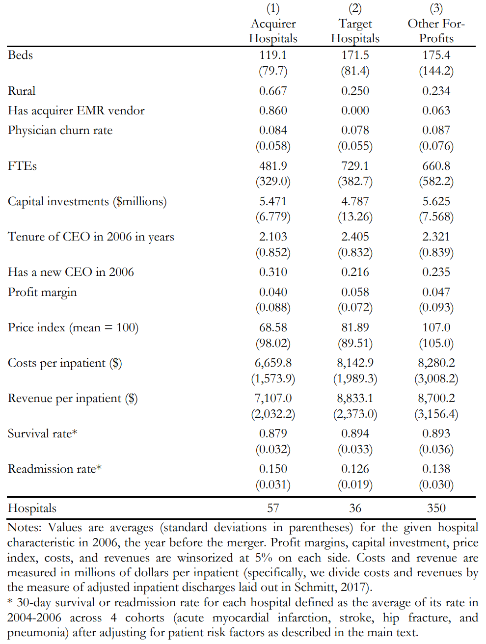
Figure 11.5: Table 1 from Gaynor et al (2021). Descriptive Statistics on Acquirer, Target, and Other For-Profit Hospitals in 2006.

Questions:

• What numbers strike you as surprising in table 1?
• What numbers in table 1 suggest that the target hospitals might be a desirable target for the acquiring firm?
• One of the stated goals of the proposed merger was to install a uniform electronic medical record, EMR, system. Was that goal accomplished?

Figure 11.6 tells us: Yes, to some degree or with mixed success.

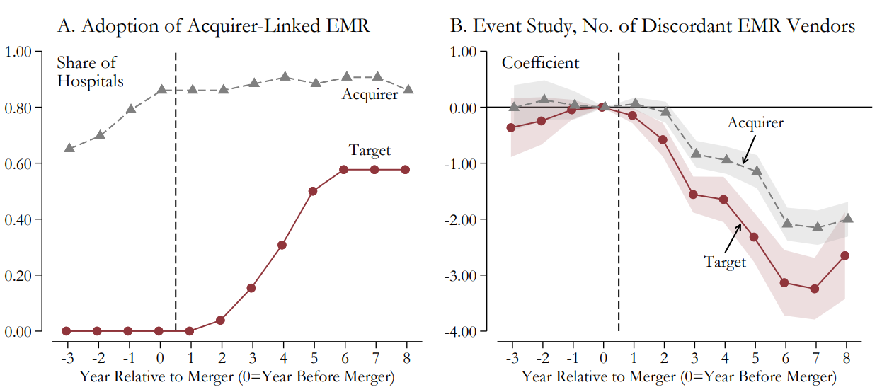
Figure 11.6: Figure 1 from Gaynor et al (2021). Visual Evidence on Merger Effects on Hospital Inputs and Outcomes

Questions: Why would adoption of one uniform EMR system across many medial providers be a good thing, i.e., what would be the economic benefits? Are there any economic costs associated with that uniformity?

Finally, to the meat! What are the economic effects of the merger?

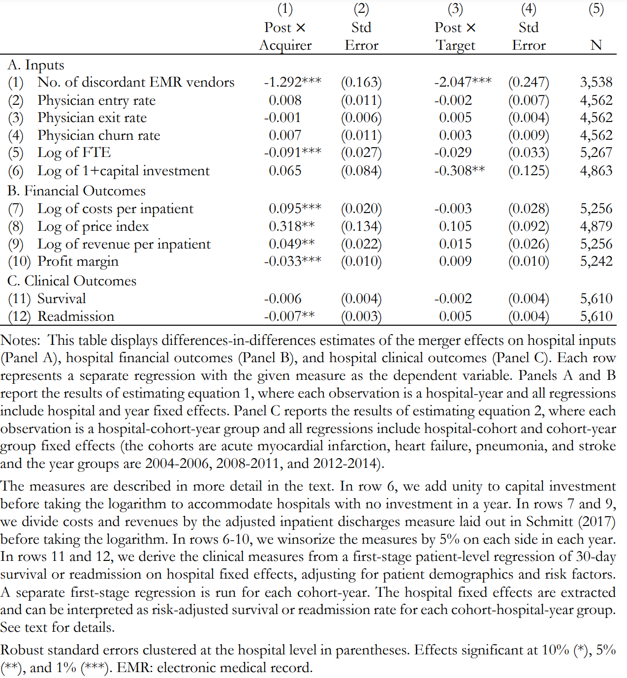
Figure 11.7: Table 2 from Gaynor et al (2021). Effects of Merger on Inputs, Financials, and Clinical Outcomes.

Capital investment in the target went down.

Apart from that effect, there are basically no other measurable effects in the target on economic or health outcomes. Things look different for the acquiring firm.

Costs per patient: UP!

Price index: UP!

Revenue per patient: UP!

Profit margin: DOWN!

Readmission rates: DOWN!

NO effect on survival rates.

Questions:

What are the costs and benefits of investment in the target hospitals doing down?

Should such mergers be allowed, if we had reasonably reliable information on merger outcomes, BEFORE the mergers take place?

What kinds of information regarding merger outcomes can we reasonably expect to have BEFORE the merger?

11.4.3 More General: Mergers in Health Care Sector

https://www.nber.org/system/files/working_papers/w17208/w17208.pdf

The literature on mergers of rivals in healthcare clearly establishes a positive relationship between mergers and prices. That means prices go UP after a merger of rivals. But this does not necessarily mean that consumers are hurt by mergers.

If prices of t shirts went up after a merger or rival t shirt producers, then consumers’ surplus would definitely decrease, and consumers would be hurt. But a price increase in health care is different. In health care most financial transactions between the health care providers and the clients/customers are intermediated by the health insurance sector. The effect of an increase in the price of health care depends on whether the insurance companies pass the price increase on to their customers in the form of higher insurance premia. If insurance premia are increased because of a merger, we would be sliding up the demand curve for health insurance. In that case health insurance coverage would decline. It turns out that the more competitive the health insurance market is, the larger the drop in health insurance coverage due to mergers. And it turns out that the biggest losers from such price increases are low income and minority populations.

In health care we can also ask: What are the effects of (changes in) concentration on quality of health care. This is exactly what is done in this paper. In a data set spanning from 1985 to 1994 Kessler and McClellan, they study the effect of firm concentration on outcomes for nonrural Medicare recipients who have been hospitalized for treatments of new heart attacks. The health care quality is measured by one year mortality.

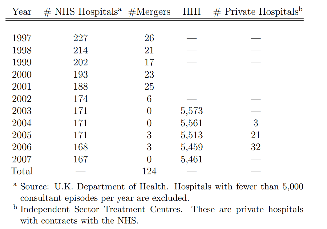
Figure 11.8: Table 2 from Gaynor and Town (2011). Hospital Market Structure, England, National Health Service, 1997-2007.

Figure 11.8 presents data on what the customer side of that market looks like. Notice among things the large but declining mortality rates. These rates drop over a relatively short period from 40% by almost a fifth.

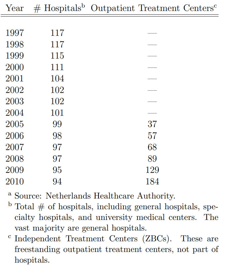
Figure 11.9: Table 3 from Gaynor and Town (2011). Hospital Market Structure, The Netherlands, 1997-2010

Figure 11.9 illustrates the rising concentration in the health care industry. This can be measured by the Herfindahl Index, or, alternatively, by the distance from domicile to the treating hospital. As is clearly visible, there is a marked increase in concentration.

What are the results?

How do expenditures per treatment change with concentration?

There is not much action in the 1980s. After 1991 things change.

Treatment in the most competitive areas was cheaper than in the least competitive areas with a difference of about 8% between the highest and the lowest Herfindahl Index quartiles.

And:

One year mortality in the least competitive areas was 1.4% higher than in the most competitive areas.

So, the punchline is:

Hospitals in highly concentrated markets spend more and have worse outcomes.

That does not look like allowing higher concentrations through mergers is in the best interest of the patients: It is never a good idea to have to pay more for a higher chance of dying.

https://www.jstor.org/stable/258700

11.5 Product Differentiation

In this section we will focus on product differentiation. We will completely abstract from price considerations. This does of course not mean that price considerations do not matter. We will abstract from these considerations in order to get a better understanding of strategic product differentiation aspects.

So here is our model. Let us be mindful that this is an abstraction.

There are two vendors selling hotdogs on a one mile stretch of Main Street, USA. The hotdogs sold by the two firms are identical. They are purchased from a common franchise, HotDoggityDog. The city requires that the hotdogs are sold at 3 bucks a piece. Customers are uniformly distributed along that one mile stretch of street. All customers will purchase from the closest vendor.

The only choice variable or strategic variable is:

Where to locate the cart?

This is illustrated in Figure 5 below. In that figure there are two firms, one located at 1/4, the other one located at 3/4. Since each customer purchases from the nearest vendor, firm 1 will get the half of the market that is located to the left and firm 2 will get the other half of the market. The customer that is located at 1/2 is the marginal customer. That customer is indifferent between purchasing from firm 1 and from firm 2.

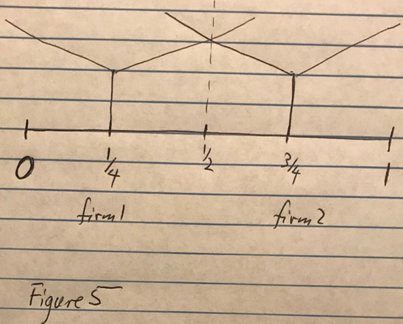
Figure 11.10: oligopoly08

Just because each firm gets half of the market does not imply that this is an equilibrium!

Suppose you are firm 2 and I am firm 1. If I am located at 1/4, what would be your best response to that?

Certainly not, 3/4! You can do better than 3/4, where you get 1/2 of the market.

If you move slightly to the left from 3/4, the marginal consumer will also move to the left and you get more than 1/2.

How far to the left should you go? If you go just to the right of 1/4, you will get almost 3/4th of the market.

That is certainly better than 1/2, don’t you think!

This sharp drop-off or increase in profit as one move just a bit away from the other player is illustrated in Figure 6 below.

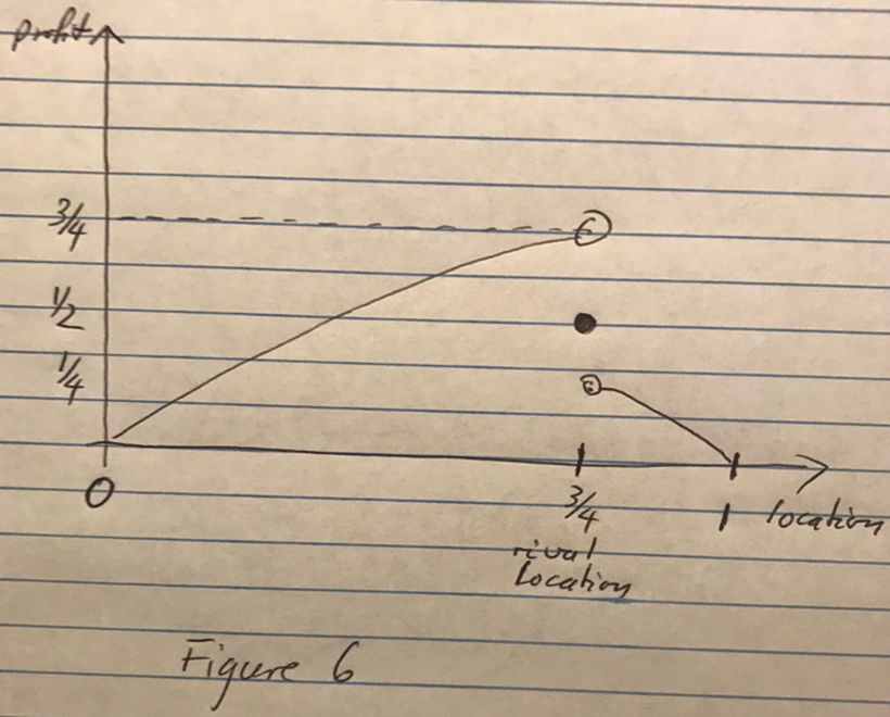
Figure 11.11: oligopoly09

But the story does not end there.

If you locate just to the right of 1/4, then it will be in my best interest to locate just to the right of you. In that case, I get almost 3/4th of the market.

But then you will move also.

We are not at equilibrium yet. Where is the Nash equilibrium in this game? If both players are located at 1/2, each player gets 1/2 and no player has any incentive to move away. As soon as player 1, say moves away from 1/2, player 1s profit drops.

This is to say:

Player 1’s best response to player 2 choosing 1/2 is 1/2 And Player 2’s best response to player 1 choosing 1/2 is 1/2

Bingo! Shangri La! Nash equilibrium!

11.5.1 Political Interpretation

Consider now two political parties or candidates that are running for elected office in the US. The election system in the US is a first past the post system; you got to get 50% plus one vote to be elected. The objective of the candidates might be to maximize the probability of getting elected or it might be to maximize the vote share. In either case the candidate chooses a position on the left-right political spectrum. What is the equilibrium in this political game?

If all voters participate in the election, the Nash equilibrium location of the two parties is indeed in the middle, where the median voter is located. Each candidate gets half of the vote. The best any candidate can do is ensure a tie.

What can we say about the kinds of candidates we get? Well, such candidates have been described as Tweedledee and Tweedledum.

Such candidates are the same, at least in the policy dimension. These candidates may differ in other dimensions, their charisma, their looks, their ability to lie with a straight face, their fund-raising ability, etc.

But on the policy dimension, they are the same. So, if a voter cares mostly about the policy, and some voters might, that raises the issue.

Why participate in the election at all?

How could this decision to vote or not be impacted by the political stance of the candidates/parties? Consider Figure 7.

In Figure 7, we have two political candidates who have stated out positions at ¼ and at ¾. Who might cast their ballot and who might not?

Voters at the very left end might not cast their ballot. They are too fat to the left, or another way of saying the same thing, the candidates, both candidates are too fat to the right. These voters on the far left may be “alienated” from the political process and, therefore, decide not to cast their ballots.

The same hold for voters on the far right. For them the candidates are to far to the left, and they may feel “alienated” from the political process as well and not cast their ballots.

There is one more group of voters who might not cast their ballots. These are the voters who are in the middle of the spectrum, the moderates, the independents. For a voter in the middle, the policies from candidate 1 are as far away from their preferred points as the policies from candidate 2. Both policies are equally good or bad. So why bother incurring the cost of casting a ballot.

These voters in the middle, while not alienated like the voters at the ends of the spectrum, refuse to cast their ballot because they are “indifferent”.

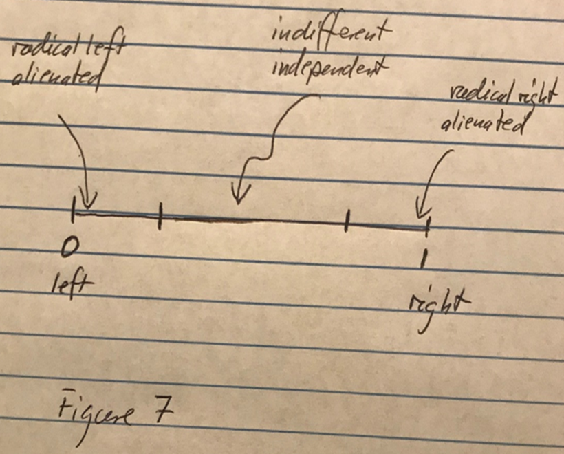
Figure 11.12: oligopoly10

These patterns of not voting will induce candidates to move away from the center. The candidate who moves away from the center can capture some of the left or right alienated voters and this hope to get over the 50% needed for election.

There is another reason for candidates not to turn into Tweedledee and Tweedledum. In the US, general elections are typically preceded by primaries. The primaries are typically closed to party members. There is a Republican primary and there is a Democratic primary.

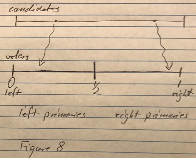
Figure 11.13: oligopoly11

Each primary will, somehow, select a candidate from that political part of the political spectrum. Once these candidates then run in the general election, they are not centrists. They have been selected from/by their party base.

In the general election, they have to appeal to the centrists. There are, at least, two ways of doing this. 1. The candidate can move more toward the center. Thereby running the risk of alienating the (radical) party base. That is of course risky. And such moves might not be credible. 2. Each candidate may accuse the other candidate of being

Radical Out of the Mainstream Un-American Socialist Fascist

If those labels stick, bingo I have won.

(But, parenthetically, and my personal opinion, the country has lost.)

11.6 More Firms!

Back from Political Science, to Economics, same game, but now with three firms. We see, in Figure 9 below, that things get just a tad more complicated. In the figure below, the three firms are located apart, roughly equally spread out.

Claim 1: That is not a Nash equilibrium location. To see this, just realize that firm 3 could increase their pay-off if it moved to the left. How far? Of course, as close to firm 2 as possible. Something like this is true for firm 1 as well: Move to the right as close as possible to firm 2. So, the location pattern indicated in Figure 9 cannot be an equilibrium.

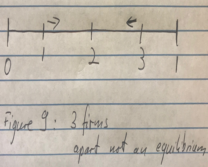
Figure 11.14: oligopoly12

Claim 2: All three firms located at ½ smack dab in the middle cannot be a Nash equilibrium either. If all firms are in the middle, each firm gets 1/3 of the market. One firm can move just a little to the right (or the left, it does not matter) to get almost ½. So, this concentration cannot be an equilibrium either.

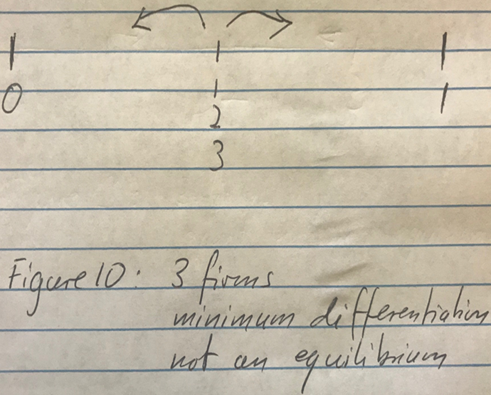
Figure 11.15: oligopoly13

Claim 3: The Nash equilibrium here involves what we call “mixed strategies”. A mixed strategy is not a fixed location, not one fixed number. It is a probability distribution. This concept should be familiar from the PKs in soccer. If you shoot a PK in soccer, you want to mix it up. If you always pick lower right corner of the goal, the goalie will know, and you will not be very successful. Hence you mix it up, you pick a mixed strategy.

How about 4 firms? This is illustrated in Figure 11 and left for an exercise.

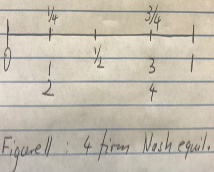
Figure 11.16: oligopoly14

Finally, let us consider a different entry and timing assumption. In the previous examples the number of firms was fixed. There was no (free) entry. Also, all firms made their location decisions simultaneously.

Now, let us assume:

• there are many potential entrants into a market
• entry decisions are made sequentially
• each firm has a fixed cost of entering/operating

These are the fundamental assumptions. There is one more assumption that has to be made: When firms enter sequentially, some firms will enter early, and some firms will enter later. When some firms enter early, they must have or form some expectations about what other firms who enter later will do, where they will locate.

If the early entrants don’t form such expectations, it is easy to see that they run a high risk of being cooked. Who wants to be cooked?

So, what shall we assume about this expectation formation?

We shall assume that firms will form rational expectations. Rational expectation here means that all early entrants, will forecast what locations all future entrants will pick. So, without any uncertainty this is really perfect foresight.

Is that a reasonable assumption? In that model: YES!

Why?

Any firm who is potential entrant j can forecast what any future entrant (j + s) will do, just by putting oneself in the shoes of entrant (j+s). This is nothing but the power and insight of Nash equilibrium. Since there is a fixed cost, and since the market is finite, there will be a finite number of firms.

Since there is a finite number of firms, there will be a last entrant and there will be a penultimate entrant. So put yourself in the shoes (boots, heels, flipflops, sandals) of the penultimate entrant. You don’t have to be a genius to figure out where the last entrant goes. Given that information you, as the penultimate entrant, will choose the nest location for you.

So given the location decision of the last two entrants, the third to last entrant, who takes as given the locations of all the previous entrant, will make rational forecast of what the last two entrants will do, when making its location decision.

So, we work our way backwards to the very first entrant.

You are right, this is just a form of backward induction.

So, what does the Nash equilibrium location in this game look like?

Firms will be spread out evenly along the entire spectrum. The space between each pair of firms is determined by the fixed cost. You must have enough of the market to cover your fixed cost. How the location choices are happening in this sequential game is illustrated in Figure 12 below. The first firm to enter will never pick a location “in the middle”. If it were to do so, it would run the risk of being squeezed on the right and the left and hence not being able to cover its fixed cost. In fact, it will be in the interest of the follower firms to do exactly that.

In order to avoid being squeezed the first firm will enter at one of the two ends of the spectrum just far enough away to cover its fixed cost. The next firm to enter will in a sense follow a similar strategy: Locate near the edge of the remaining spectrum, on either end, so it can cover its fixed cost. Two possible location patterns are illustrated in Figure 12.

Ultimately, where exactly each individual firm is located is immaterial. What matters is that all firms are roughly equally spread out and that the entire spectrum is covered.

Wandering down the ready to eat breakfast cereal aisle in your favorite grocery store might remind you of the Nash equilibrium locations in the figure below. The “space” is filled out it seems, completely, with ready to eat cereal of all flavors, fiber content, sugar content. It seems impossible for any entrepreneur to enter that thicket profitably.

Breakfast cereal is not the only example of a market that looks like Figure 12 below.

How about: - Sweetened Iced Tea - Gas stations in Bloomington or in Fort Wayne for that matter. - Cat/dog food - Others

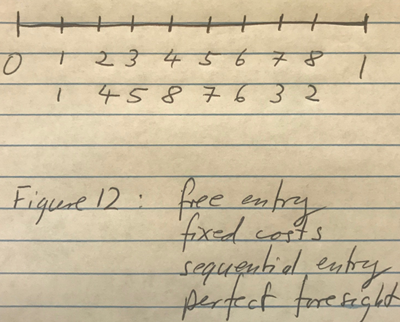
Figure 11.17: oligopoly15

11.7 Glossary of Terms

Bertrand equilibrium: The equilibrium in an oligopoly when all firms have price as the strategic variable.

Cournot equilibrium: The equilibrium in an oligopoly when all firms have quantity as the strategic variable.

Heterogeneous goods: These are goods that are different in some way by taste, color, location, durability or any other characteristics. Or at least they are at purchase perceived to be different.

Homogeneous goods: These are goods that are the same by taste, color, location, strength, and any other relevant characteristic. Or at least they are at purchase perceived to be the same.

Horizontal differentiation: This refers to different types of goods such as different degrees of sweetness of the iced teas. There is no sense that one variant is better than the other; they are just different and different consumers prefer different variants.

Location game: A game where a relatively small number of firms strategically choose a location. This could be in geographic space or in “product space”.

Market concentration: This is a measure of how many or how few firms are in a particular market.

Rational expectations: Expectations formed by agents in a model that turn out to be true, in the model, at least in an expected value sense.

Vertical differentiation: This refers to different levels of quality, where most consumers agree that some goods are better than others, such a durability of a pair of jeans, or the gas mileage of a car, internet speed,etc.

11.8 Practice Questions

11.8.1 Discussion

1. Is the location for both firms at ½ in the two-player game efficient? Think of “transportation costs”.
2. In the location problem of the two firm location game, where is the efficient location of the two firms?
3. In the location game described above, suppose there are 4 firms. What is the Nash equilibrium location? Explain.
4. In the 4 firm location game, what is the efficient location? Explain.

11.8.2 Multiple Choice

1. Imagine a duopoly where two firms sell an identical product and play a one shot Cournot Nash Game. If form 1 increases its output, then

   A. It is rational for firm 2 to produce more
   B. It is rational for firm 2 to produce less
   C. It is rational for firm 2 to leave its output constant.
   D. It is rational for firm 2 buy up firm 1

2. Imagine an oligopoly where three firms sell an identical product and play a one shot Cournot-Nash game. If firm 1 increases its output and firm 2 keeps its output constant, it is rational for firm 3

   A. To produce more
   B. To produce less
   C. To leave its output constant
   D. To buy up one of the two other firms.

3. Imagine an oligopoly where three firms sell an identical product and play a one shot Cournot-Nash game. If firm 1 increases its output and firm 2 decreases its output by the same amount, it is rational for firm 3

   A. To produce more
   B. To produce less
   C. To leave its output constant
   D. To buy up one of the other two firms.

4. Imagine a duopoly where two firms sell and identical product and play a one-shot Bertrand-Nash game. If firm 1 increases its price, it is rational for firm 2

   A. To increase its price
   B. To decrease its price
   C. To keep its price constant
   D. To buy up the other firm

5. Imagine an oligopoly with 3 firms that sell an identical product and play a one-shot Bertrand-Nash game. If firm 2 raises its price,

   A. It is rational for firm 1 to raise its price
   B. It is rational for firm 1 to lower its price
   C. It is rational for firm 1 to keep its price constant
   D. We don’t have enough information to decide what is rational for firm 1.

6. Imagine three firms playing a Bertrand-Nash price game for 20 rounds. The demand function in each round is given by P = 10 – Q, where Q is total industry output. All three firms are very rational. We can expect

   A. The price to be 10 in each round
   B. The price to be 5 in each round
   C. The price to be equal to marginal cost in each round
   D. The price to be equal to zero in each round

7. Imagine that 2 firms play a location game on a circle, not the disk, the circle. The circle has circumference length 1. Prices are fixed. The firms choose location simultaneously.

   A. There is exactly one Nash equilibrium location, and the firms have unequal market share
   B. There are many Nash equilibrium locations and both firms have unequal market share
   C. There is exactly one Nash equilibrium location, and the firms have equal market share
   D. There are many Nash equilibrium locations and both firms have equal market share.

8. Consider an oligopoly with 10 firms playing a Cournot-Nash game for one period. The firms are selling a homogeneous product. If 4 of the 10 firms merge, we can expect

   A. The price to increase
   B. The quantity to decrease
   C. Overall industry profit to increase
   D. All of the above

9. In problem 8 above, assume instead that the firms are selling differentiated product. All other aspects of the industry are the same. Then after the merger we would expect

   A. Prices to increase
   B. Overall quantity sold to decrease
   C. Overall industry profit to increase
   D. All of the above

10. Imagine two vendors of a consumer product to be located at ¼ and at ¾ of a one-mile-long street in Littlecity. The city passes a zoning law that forces the two firms to relocate more toward the center of the street. After this law is passed, we would expect

    A. Price competition to decrease
    B. Price competition to increase
    C. Price competition to stay the same
    D. Profits to rise