9 Monopoly

In this chapter we will learn:

Fundamental causes that differentiate monopolistic outcomes from competitive outcomes.
Differences between monopolistic and competitive outcomes, including their (in)efficiency properties.
Effects of policies including subsidies and price ceilings on the efficiency properties of monopolistic equilibrium.
Explain different kinds of price discrimination and how such pricing practices can enhance profitability.
Explain how two-part tariffs increase profit relative to uniform pricing.

9.1 Introduction

In the previous chapters we have studied competitive markets. These were markets with many buyers and many sellers. I fact we have so many firms and so many households that no single individual firm and no single individual household can influence the price.

A monopoly is at the very opposite end of the spectrum. Instead of having a huge plethora of firms in the market, in a monopoly there is exactly one firm. Only one.

Of course, this is an extreme case. There are indeed some industries that fit that bill. But some of the insights from this extreme case will carry over to other cases that are not quite that extreme, where some, usually a small number of, firms have what we call market power.

Since there is only one firm in the market, it will face the market demand function. Whatever the market demand function happens to be, that is what the monopolist has to work with. That does imply that the monopolist realizes the following: If the price goes up, the quantity demanded goes down. If the price goes down, the quantity demanded goes up. In other words: For the monopolist there is no way of getting around the law of demand. We sometimes hear in popular discussions that the monopolist is free to set ANY price in a completely unconstrained manner. That would be false. The monopolist has to “obey” the law of demand in its market.

By contrast: in a competitive market, each firm faces a completely horizontal demand curve. This is a consequence of the assumption that, in a competitive market, the price is given by the market and that no firm can influence the price. Rather, at whatever price the market sets, each firm can sell as much as it likes. At the market determined price, each firm can sell its profit-maximizing quantity.

This difference between a firm in a competitive market and a monopolistic firm is fundamental to all differences between these two types of markets. All differences between these two types of markets hinge on this one difference. [I cannot think of another way to say that this is important.] Figure 1 illustrates this one fundamental difference. Figure 9.1’s Panel a depicts the demand that each individual firm in a competitive market face. It is flat. Panel b depicts a downward sloping demand function that a monopolist is facing.

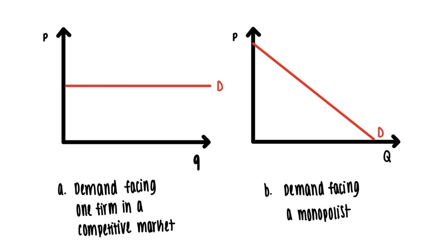
Figure 9.1: Fundamental difference between competitive and monopolistic markets.

In Figure 9.2 below we are starting to figure out the behavioral differences between a competitive firm and competitive markets on the one hand and a monopoly on the other hand. In Figure 9.2, imagine that for some reason, whatever that reason is, the monopolist is charging $10 and at that price, the monopolist can sell 10 units. Then the total revenue is $\$100$. If the monopolist wanted to sell more units, the price would have to be decreased.

Why? The Law of Demand. The demand function is downward sloping.

Concretely, suppose the monopolist wants to sell 11 units and not 10. As indicated in Figure 9.2, the price would have to come down to $\$9.50$ in order to entice consumers to buy 11 units. If 11 units are sold, the total revenue is the price, the new price, $\$9.50$ multiplied by the quantity, 11. That is $\$104.50$.

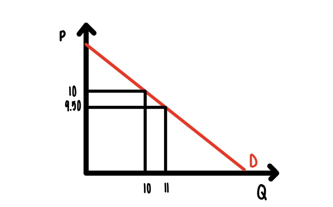
Figure 9.2: Marginal revenue is below demand

The extra revenue from selling that 11 unit, the last unit is $\$4.50$. That is far less than the price of $\$9.50$. What we have shown with this example, and what is true in general is that for the monopolist, marginal revenue is below the price, below demand.

This is radically different from competitive markets. Imagine you are selling a boring t shirt for $12 in a competitive market. For each t shirt you sell the extra revenue you get is $\$12$.

For the first shirt you get $\$12$.
For the second shirt you get $\$12$.
For the third shirt you get $\$12$.

Punchline: In a competitive market, the marginal revenue is the price. It is constant, regardless of how much stuff you sell.

Why is the marginal revenue in a monopoly below demand (the price), while in a competitive market the marginal revenue is equal to the price. Always!

The fundamental difference between a monopolist and a competitive firm is that the monopolist faces a downward sloping demand curve: In order to sell more, the price must come down, The (Iron?) Law of Demand strikes here. But what is crucial is: Price must come down, not only for the last unit sold, the 11th unit in the above example. Rather, the price must come down for ALL units, in the above example, the first 10 units as well.

Since the price must come down on all units, on all 11 units, it is not surprising that marginal revenue is small, in particular below demand.

We can further illustrate this with a numeric example. Suppose that demand for a particular product is given by

\[P = 10 – Q\]

where $P$ is the price and $Q$ is the quantity. Then in the simple table below we can easily calculate for each quantity, the price derived from the demand curve. This is done by just substituting the quantity into the above demand function and then reading off the price. If the quantity is 3, the price is $\$7$.

The second step is to calculate total revenue. That is just multiplying the price and the quantity. In the table below, simply, row by row, multiply the value in column 1 with the value in column 2. In the third row, 3 times $\$7$ yields $\$21$ for total revenue.

How do we get to marginal revenue? Using the definition or marginal revenue, we just go row by row. How much extra revenue do we get as we go from row 3 to row 4, as we sell the fourth unit? As you increase the number of units sold from 3 to 4, total revenue goes up from $\$21$ to $\$24$. The extra revenue from selling that last unit, that forth unit is 3. The marginal revenue from selling the fourth unit is $\$3$.

Q	P	TR	MR
1	$\$9$	$\$9$	$\$9$
2	$\$8$	$\$16$	$\$7$
3	$\$7$	$\$21$	$\$5$
4	$\$6$	$\$24$	$\$3$
5	$\$5$	$\$25$	$\$1$
6	$\$4$	$\$24$	$-\$1$
7	$\$3$	$\$21$	$-\$3$
8	$\$2$	$\$16$	$-\$5$

Notice two things:

Marginal revenue can be negative. That is often true when the monopolist sells too much.
If you compare columns 2 and 4 you see that as output increases by one unit, the price, read off from the demand function, goes down by one unit. But marginal revenue goes down by two units. This pattern will always prevail when demand is a linear function.

We can state the general principle:
If demand is of the form
\[ P=\alpha-\beta Q\]

where α and β are some arbitrary parameters, then the marginal revenue function is given by:

\[MR = \alpha - 2 \beta Q\]

Another way of saying this is: If the demand function is any linear function, then the marginal revenue function is also linear, and it is twice as steep.

9.2 Monopoly Pricing

Much of economics is actually very simple. It follows a few very simple rules. In the chapter on Rational Choice we learned:

Rational behavior entails equating marginal cost and marginal benefit of the action.
For the particular action we just have to know what he is marginal cost of the action and what is the marginal benefit of the action.

For a monopolist the marginal cost of producing is clear, it is just the marginal cost. This is the same for any firm. The marginal benefit of producing is the marginal revenue obtained from selling stuff. So, for the monopolist, rational profit maximizing behavior is

Equate marginal revenue to marginal cost.

How this works is illustrated in Figure 9.3.

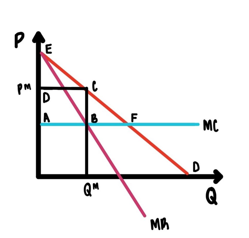
Figure 9.3: Profit maximization by a monopolist

In Figure 9.3, the demand function is linear and downward sloping. The marginal revenue is below the demand function, and it is twice as steep. The marginal cost function is drawn horizontally, indicating constant marginal cost or constant returns to scale. This does not have to be that way. This is done purely for simplicity of exposition.

Equating marginal revenue to marginal cost yields the monopoly output which we denote $Q_M$. At $Q_M$ marginal revenue is equal to marginal cost. This maximizes profit. [You should be able to convince yourself now that this is indeed so.]

So, we have determined how much the monopolist produces, IF profit maximization is the goal. We need to determine the price. In order to find the price, we simply start with the quantity $Q_M$ and go up along a vertical line until we hit the demand function. Why? One we hit the demand function we can go over to the vertical axis and read of the corresponding price. We label this price $P_M$.

$P_M$ is the highest possible price the consumers are willing to pay so that exactly $Q_M$ units will be sold. So, $Q_M$ is the profit maximizing quantity and $P_M$ is the highest possible price that is consistent with the profit maximizing decision.

So far so good. What else can we get out of Figure 9.3?

The point $F$ is the efficient point. This would be the equilibrium if this market were efficient. But it is not.

The area of the triangle $DCE$ is consumers’ surplus. This is smaller than what it would be if the market were competitive.

The area of the rectangle $ABCD$ is the monopolist’s profit. Why? For each unit between $0$ and $Q_M$, the price is above the marginal cost. That vertical difference is the profit made on each unit. Add up all these vertical differences from $0$ to $Q_M$ and you got the profit, given by the area of the rectangle $ABCD$.

That leaves us with the area $BFC$. If the market were competitive, this area would be part of consumers’ surplus. But the market is not competitive. That area is also not part of profit.

The area $BFC$ is not part of consumers’ surplus. It is not part of profit. It has been lost. It has disappeared. We call this area the

Deadweight Loss of Monopoly

This area is really a loss to society. You see, anywhere between $Q_M$ and $F$, some consumer is willing to pay more for the product than is required to produce it. For each unit in that region that is not sold, there is a loss to society, an opportunity for welfare/utility/pleasure foregone. Adding up all these losses over all goods between $Q_M$ and point $F$ generates the area of the triangle $BFC$. This is literally a potential welfare that has been lost to the power of monopoly. We should think of this welfare loss as real resources that could have been useful to some consumers, but since we are dealing with a monopoly here, these resources will never be produced. These resources, potential as they might be, have just gone up in smoke.

9.3 Mark-ups

It is clear from Figure 9.3 that for a monopolist the price is above marginal cost. This is a fundamental difference to competitive markets, where prices are always equal to marginal cost.

Often, we will use a measure of the distance of price to marginal cost as a measure of market power. Market power here refers to the ability to elevate price above marginal cost.

We will define \[\text{Mark-up} = \frac{\text{Price}}{\text{Marginal Cost}}\]

We will refer to this as the “price-marginal cost mark-up” or just the “mark-up” for short.

In some cases, mark-ups are small, in others they are large.

As you make a donation of $\$1,000$ to your favorite charity, you discover that the credit card you are planning to use will charge you $\$30$ for the transaction. This charge strikes you as extremely high, especially since your estimate of the marginal cost of “booking” this transaction must be very close to zero.

A bottle of wine in a restaurant might set you back $\$50$, even though you can get that same wine for $\$12$ at the grocery store.

There are many other examples of high mark-ups. You are invited to make a list.

The size of the mark-up, of course, depends upon the elasticity of demand:

High elasticity, low mark-up. Low elasticity, high mark-up.

The monopolist is constrained by demand, by the elasticity of demand. There is no escaping that. If there are lots of good substitutes, the elasticity is high, and the markup is low. But if there are few substitutes, then the elasticity is low, and the mark-up is high.

When businessmen are asked what is the secret to success, they sometimes say things like:

Build a moat around your business.

That means make sure that there are no competitors that can offer similar products and thus encroach on your territory and thus minimize your mark-ups. This makes perfect sense. The fewer substitutes there are for your product or service, the bigger the mark-up and, of course, the bigger the profit and the better the French red wine you might be drinking.

How to obtain or build such a moat?

One of the most commonly used methods is advertising and/or branding. If you are successful in your branding, you will distinguish your product from that of competitors, perhaps for real or perhaps only in the mind of your clients. But that is enough. If your clients think that your product brand is unique and special, they will not be as satisfied with the possible substitutes and they will be willing to pay a premium.

Then you have your moat.

The punchline that the price-marginal cost mark-up is inversely related to the elasticity of demand also has implications for optimal tax policy.

When demand is relatively inelastic, the monopolist can raise the price, without fear of having the quantity demanded go way down.

The same force actually informs optimal tax policy. Imagine that your government needs to raise a certain amount of funds for a particular project. Which goods should be taxed? Goods with elastic demand or goods with inelastic demand?

The relationship between mark-ups and the elasticity of demand suggests that it is optimal to tax goods with inelastic demand more than goods with elastic demand.

If you want to minimize the deadweight loss of taxation, you ought to make sure that the consumption response to an increase in the tax is not very large. After all, it is the consumption response, the reduction in consumption, that hurts the consumers. The more elastic is demand, the bigger the reduction in consumption as the tax rate is increased; and the bigger is the welfare loss to consumers. Therefore, it is more desirable to tax goods whose demand is more inelastic. The rule is:

If a fixed amount of revenue has to be raised, the optimal tax rate is inversely related to the elasticity of demand.

That is one reason why taxes on tobacco are so high. It is harder to imagine products whose demand is more inelastic than the demand for the super addictive nicotine.

There is one industry that also seems to have super high mark-ups and therefore super high profits: The non-profit hospitals in Indiana.⁵⁰

Sometimes it is convenient to express profits as a fraction of revenue. This is done in the table below. These numbers are really astonishing. For-profit Walmart has a profit ratio of about 3% to 4%. Of course, this varies from year to year. But the ballpark numbers are around 3-4%.

How do the non-profit hospitals stack up? The table below, taken from the Ball State Report shows for the 13 hospitals listed in that table profit rates range from 49% down to about 19%. Even for the 13th lowest profitable hospital, the profit rate is higher than Walmart’s profit rate by a factor over 4!

Figure 9.4: Hospital Profit Rates.

This finding was very controversial. That is not a surprise.

But the numbers in the Ball State report are what they are, and they show what they show.

Often when I introduce myself as an Economist, the first question is: Are you a micro or a macro economist.

My response often is: The distinction between micro and macro is vastly overblown. There is only Economics. When you look at the profit rate of one single hospital, like St. Vincent Carmel Hospital, with a profit rate of 38%, that would be micro.

But the report also points out that the five most profitable non-profit hospitals made a profit in 2017 that is equal to 8% of Indiana GDP for that year. That is a staggering number. And that is macro.

This is just another way of looking at the same numbers that we would be looking at in micro. Micro and macro are here, and very often, intertwined.

So, you are making huge profit margins. You are sitting on a pile of cash. What to do with it?

One organization that has to deal with this issue is the NCAA.⁵¹

In general, there are only two collegiate sports that make money: men’s basketball and football. The profits from these two sports can be large, especially of the programs regularly rank in the top 20 or 25. Think Ohio State or Alabama in football and think Duke and Kansas in basketball.

So, what to do with all that profit?

One could buy better equipment for the chemistry labs.
One could have higher scholarships for graduate students.
One could have better mental health counseling.
One could have better writing services.
One could have better tutoring services.
Or one could use that profit from football and men’s basketball to fund other sports that do not generate a profit: track and field, field hockey, crew, gymnastics, etc.
Or you could just funnel the profits back into the football and men’s basketball program.

So, what is the typical practice? Out of an extra $100,000 in profit, $80,000, or 80% is funneled back into those programs. For more staff, higher salaries for staff, more equipment, better facilities.

The other 20% of profits goes to the other non-profitable sports.

The paper also documents that athlete who participate in football or men’s basketball are largely Black and come from poorer zip code areas. While participants in the other sports are more white, more female and come from richer zip code areas.

So, the NCAA basically distributes money from relatively poor Black athletes to relatively well-off white, female athletes.

You decide on the ethics of that redistribution!

9.4 Two Corrective Policies

Since there is good reason to believe in the inefficiency of monopoly, it is a good idea to think about whether there are any government policies that could eliminate that inefficiency. Both policies considered will have fundamentally different effects than in competitive markets.

The first policy we consider is a price ceiling. That is, as before, a legal limit on how high the price can go. Remember that in a competitive market, a price ceiling causes the quantity demanded to exceed the quantity supplied so that there is a shortage and so that the quantity traded actually goes down.

How this actually works in a monopoly is illustrated in Figure 9.5. In Figure 9.5, the demand function is downward sloping as usual, the marginal cost function is flat, the monopoly quantity is $Q_M$ and the monopoly price is $P_M$. Now suppose in that situation we, the government, introduces a price ceiling at the level $P_C$. Of course, this ought to be below the monopoly price. Otherwise, what would be the point.

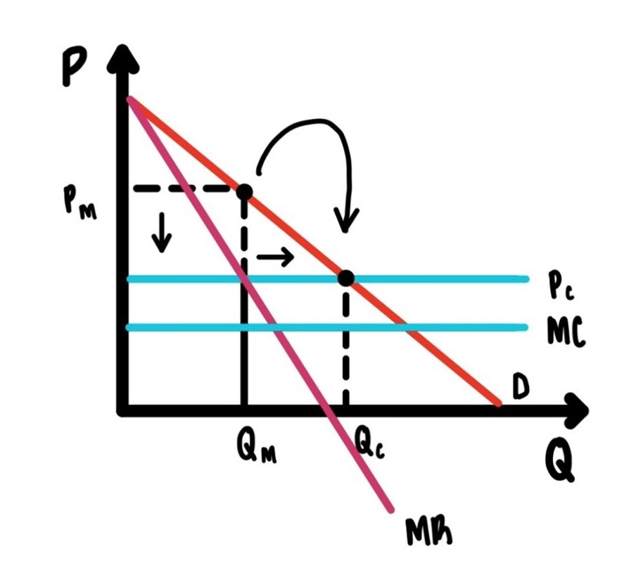
Figure 9.5: Price ceiling for a monopolist.

Once there is a price ceiling, the monopolist will produce more, the price comes down (of course), the deadweight loss of monopoly shrinks, and the market becomes more efficient.

Why? If there is a price ceiling, that ceiling becomes marginal revenue. For the first t-shirt you get $\$12$, for the second t-shirt you get $\$12$, etc. etc. etc.

Marginal revenue is above marginal cost. So, for your t-shirt you sell you make a profit. In that case you want to sell as many t-shirts are possible. At that price ceiling.

But there is a break. Eventually you will run out of customers who are willing to pay $P_C$. That determines how many units the monopolist will sell.

The profit has shrunk. In Figure 9.5 the new profit is given by the rectangle to the left of $Q_C$ and below $P_C$.

The second policy measure we consider is a per unit subsidy to the monopolist. Imagine that the government pays the monopolist $\$s$ for each unit produced. In Figure 9.6 we see that this will decrease marginal cost exactly by $\$s$.

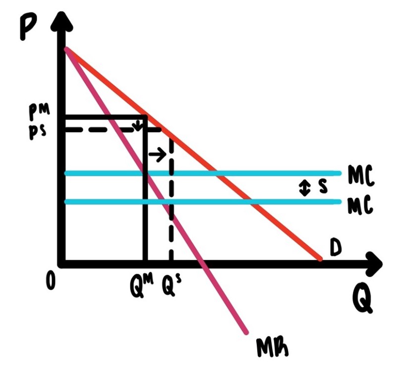
Figure 9.6: A subsidy for the monopolist

Figure 9.6 then clearly shows that as marginal cost declines the point where marginal cost and marginal revenue intersect moves to the right. The quantity sold increases. And, since demand is downward sloping, the price has to come down as well. As the price comes down and the quantity goes up, we are getting closer to the efficient allocation and the deadweight loss of monopoly declines.

This is exactly what we would want. But there is one big issue. This subsidy, like all subsidies has to be financed. Somehow. The government can raise taxes, or cut other programs, or tun a deficit. But running a deficit just means that future taxes need to be raised or future benefits need to be cut.

The big rub is this: How to convince anybody of the following:

Why on earth would we ever want to subsidize a monopolist. In the public’s eye they are making enormous problems as it is. So why subsidize them? That seems like “shipping coals to Newcastle.”
How to convince people that such a subsidy might actually increase efficiency?

Both of these seem to be tall orders.

9.5 Price Discrimination

Imagine that the monopolist can segment the markets into two parts, one part depicted in Figure 9.7’s Panel a and the second market depicted in Figure 9.7’s Panel b. In the example in Figure 9.7 we assume that marginal costs are the same in both markets.

There are lots of ways markets can be segmented in various submarkets.

Households can be divided into families and households of unrelated individuals.

IU basketball fans can be divided into students, faculty, alumni, staff, townies.

Vacationers going on a cruise can be subdivided into families with kids, singles, retired couples, retired couples from New Jersey, retired couples from Nebraska.

You get the idea. The possibilities are endless.

In some pairs of markets marginal costs might vary. In other pairs of markets marginal costs might be the same. The marginal cost of a hamburger in a restaurant is going to be the same, regardless of whether the hamburger is sold at a discount to a senior citizen. If markets are segmented along geographic lines, transportation costs might generate an inequality of marginal costs between markets.

Figure 9.7 illustrates how market segmentation can increase profits. Figure 9.7 shows one market segment in each panel.

How does profit maximization work? In market 1, equate marginal revenue to marginal cost and then read of the price. In market 2, do exactly the same thing to get the price in market 2. Since the two demands are different, it is not surprising that the two prices are different.

Business travelers pay a different price on an airplane than tourists.

Senior citizens pay less for a restaurant meal than college students.

Etc.

It is easy to see that such market segmentation is profit maximizing. Imagine, that the monopolist charges a uniform price in both markets that corresponds roughly to the average price in both markets, rather than different prices in both markets. Then we see that the profit in market 1 goes down. Profit in market 1 must go down, because the average price is not the profit maximizing price in that market. Since it is not the profit maximizing price, it must generate lower profit in that market.

The same is true in market two. The average price is also not the price that is profit maximizing in the second market. So, it must decrease profit in the second market as well.

We have learned that ANY price that is uniform across the two markets must decrease profits in both markets relative to prices in each market that equate marginal revenue to marginal cost in each market.

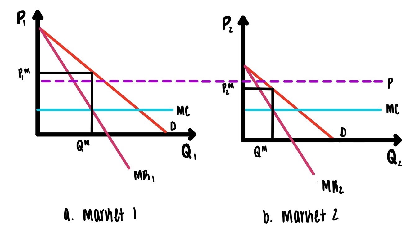
Figure 9.7: Price Discrimination via market segmentation.

The example of segmenting the market into two parts above shoes that market segmentation is a profit maximizing strategy.

Of course, segmenting markets like this is not free. In order to profit from such market segmentation, the monopolist must first be able to gather enough information. The monopolist must have information in the elasticities of demand in both markets. The price mark up over marginal cost will be determined by the elasticity of demand in each market. But that can only happen if there is information on these elasticities.

In the example above the market has been segmented into two parts. You can easily imagine segmentation in finer, smaller groups.

Imagine you are running a cruise line. Whenever a ship leaves with an empty cabin you have lost revenue. In order to fill that last cabin, you need to know how to price, and you can increase your profit by picking the profit maximizing price for each segment of the market. What could these segments be?

Single people
Single men
Single women
Single retired people
Single retired men
Single retired women
Others of course.

In the limit, as you make this segmentation finer and finer and finer, each segment will consist of one consumer only. Then each consumer will face a potentially different price. This is truly profit maximizing as illustrated in Figure 9.8.

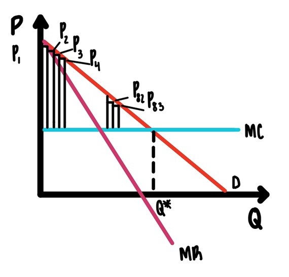
Figure 9.8: Perfect Price Discrimination.

The entire area between demand and marginal cost, now has turned into profit. There is no way profit could get any bigger.

Notice also that the resulting allocation is efficient. The allocation that results from perfect price discrimination is, in Figure 9.8, given by $Q^*$. At $Q^*$, marginal cost is equal to marginal benefit. That is efficient.

Of course, this practice of perfect price discrimination comes at a cost. This price discrimination is only possible if the monopolist knows each customers reservation price.

How might companies be able to gather information of reservation prices? Think of the Kroger shopping card, think of Amazon or Netflix or your random casino in Vegas. These companies have all kinds of information about their customers’ preferences. They could almost do personalized pricing.

9.6 Mickey Mouse Pricing

In many situations there are very large, fixed costs and marginal costs are often close to zero. The Magic Kingdom and other amusements parks come to mind. But there are other cases that are close. In such situations firms often adopt what is called a

Two Part Tariff

Sometimes a two-part tariff is referred to as Mickey Mouse Pricing, since such pricing is often used by the theme parks of the Disney Corporation. A two-part tariff simply means that the price is not ONE number but a set of TWO numbers. One of these numbers is an entry fee. The other is a price per unit of the good consumed.

How this works is illustrated in Figure 9.9. Imagine a theme park with lots of rides. There is a demand for the theme park and once inside there is a demand for the rides. Inside demand is downward sloping, as usual and marginal cost is constant and close to zero. For starters we assume all consumers are alike in the sense that they have exactly the same demand.

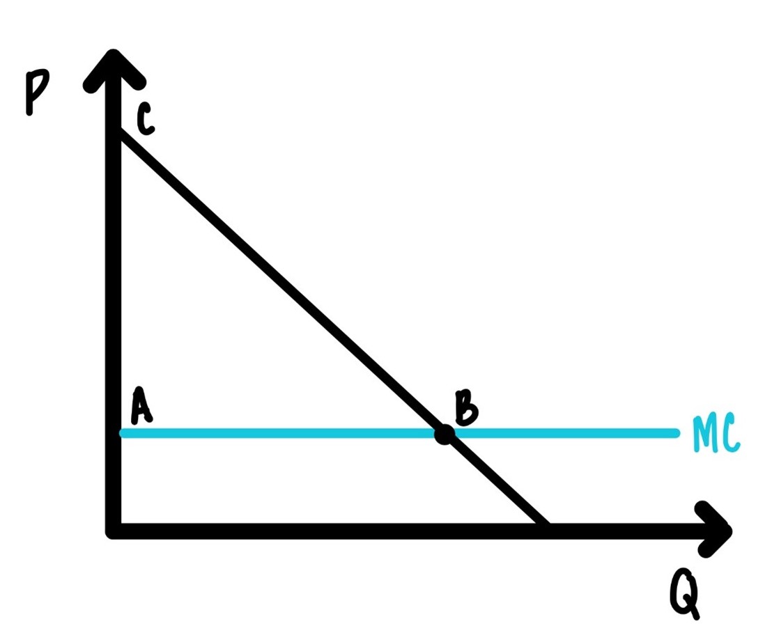
Figure 9.9: Simple two part tariff.

If the price per ride is exactly equal to marginal cost, then the area of the triangle $ABC$ is consumer surplus, the surplus of a representative consumer.

How should the monopolist charge the entry fee? The highest entry fee that the monopolist could possibly charge is a fee that is equivalent to the area of the triangle $ABC$, the area that is the entire consumer surplus. Then charge marginal cost for each ride.

Often marginal cost is really close to zero. Think of the marginal cost of you going on one more ride at some amusement park. That is really close to zero. Then it might now be worthwhile even collecting the price for an extra ride. In such cases often we see $p = 0$.

This two-part tariff maximizes profit. There is nothing the firm can do to increase its profit further.

This was a very simplified example with only one type of consumer, with identical consumers that all have exactly the same demand, the same willingness to play to the amusement park. Of course, this is not realistic. What happens when there are different types of consumers, when some consumers have a small willingness to pay, and other consumers have a large willingness to pay?

This situation is illustrated in Figure 9.10. There we have the same basic set-up as in Figure 9.9, except that there are two types of customers, one with small demand, one with big demand. It is important here to state that the monopolist knows that there are two different types of customers, but the monopolist does not know which customer is big and which is small. So, there can be no price discrimination. That means that the entry fee and the price per ride must be the same for all customers.

We will start our analysis by assuming that $p = MC$ as in the previous case. If $p = MC$, what is the entry fee?

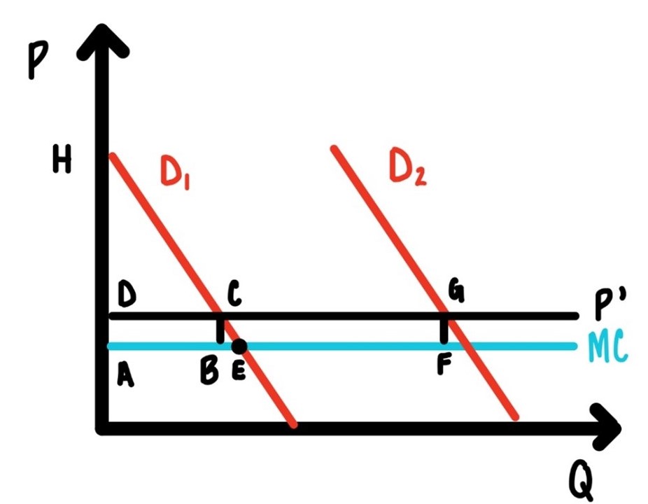
Figure 9.10: Two part tariff with multiple consumer types.

Since there are two types of customers, figuring out the right entry fee is a bit tricky. If it is too large the small customer will not come. So, it stands to reason that the entry feel will be just a bit below the consumer surplus of small consumer, i.e., the area of the triangle $AEH$.

So, will the two-part tariff be Entry fee = area $AEH$ and $p=MC$?

The answer is NO.

The firm can do a bit better if they raise the price a bit above MC to the price $p’$ and adjust the entry fee accordingly. What happens then?

The area $ABCD$ still goes to the monopolist. If the price is equal to marginal cost, then that are is part is consumer surplus that goes straight into the entry fee and in the monopolist’s pocket. Now that are is not in the entry fee, but it is part of the revenue obtained by have the price $p$ above marginal cost.

The area $ABCD$ goes into the monopolist’s pocket in any case. The monopolist does not care if he/she gets that area is part of the entry fee or as part of the price. As long as it is part of the profit.

What about the area $BEC$? That is indeed a loss to the monopolist. It used to be part of the entry fee. Now it is a loss to the monopolist, since at the price $p’$ the quantity demanded is smaller than at the price $p = MC$.

So, if this makes any sense at all, there must be a gain to the monopolist of raising the price top’ above marginal cost. What is this gain? That gain is the area $AFGD$, from the big consumer. That area is obviously bigger than the small loss of $BEC$.

The punchline is this: The profit maximizing two-part tariff has a price slightly above marginal cost, call it $p’$, and an entry fee that corresponds to the area $DCH$.

Do we actually see such pricing practices? We don’t have to go very far. Just about a block away from IU there is a bar that shall remain unnamed. That bar used to advertise

Two Dollar Tuesdays.

Two dollars to get in, two dollars for a beer. Two dollars to get in as a relatively small entry fee I am confident that there are many IU students who would be willing to pay a higher entry feel in this particular amusement park. But the profit maximizing entry fee is equal to consumer surplus of one of the smaller customers.

Two dollars per beer is slightly above marginal cost of a beer.

That practice fits the theory almost to a T.

9.7 Taylor Swift Pricing

IU will play Michigan State in men’s basketball on Feb 20, 2022. I can buy tickets for his game today, or in November, or in December, or in January, or even February 18, 2022. Whenever I buy these tickets, the price will be the same. And that price is determined now, call it $50 per seat in the nosebleed section.

That price does not change until February 20.

Should it change? Should it be the same?

How might that price change over time?

Imagine, this is pure imagination, that IU has a terrific season in November and December. Imagine that IU will beat a bunch of powerhouses on the schedule in November and in December and IU beats Michigan State at MSU.

If that is the case, what might happen to Hoosier’s willingness to pay? My guess would be that willingness to pay will rise.

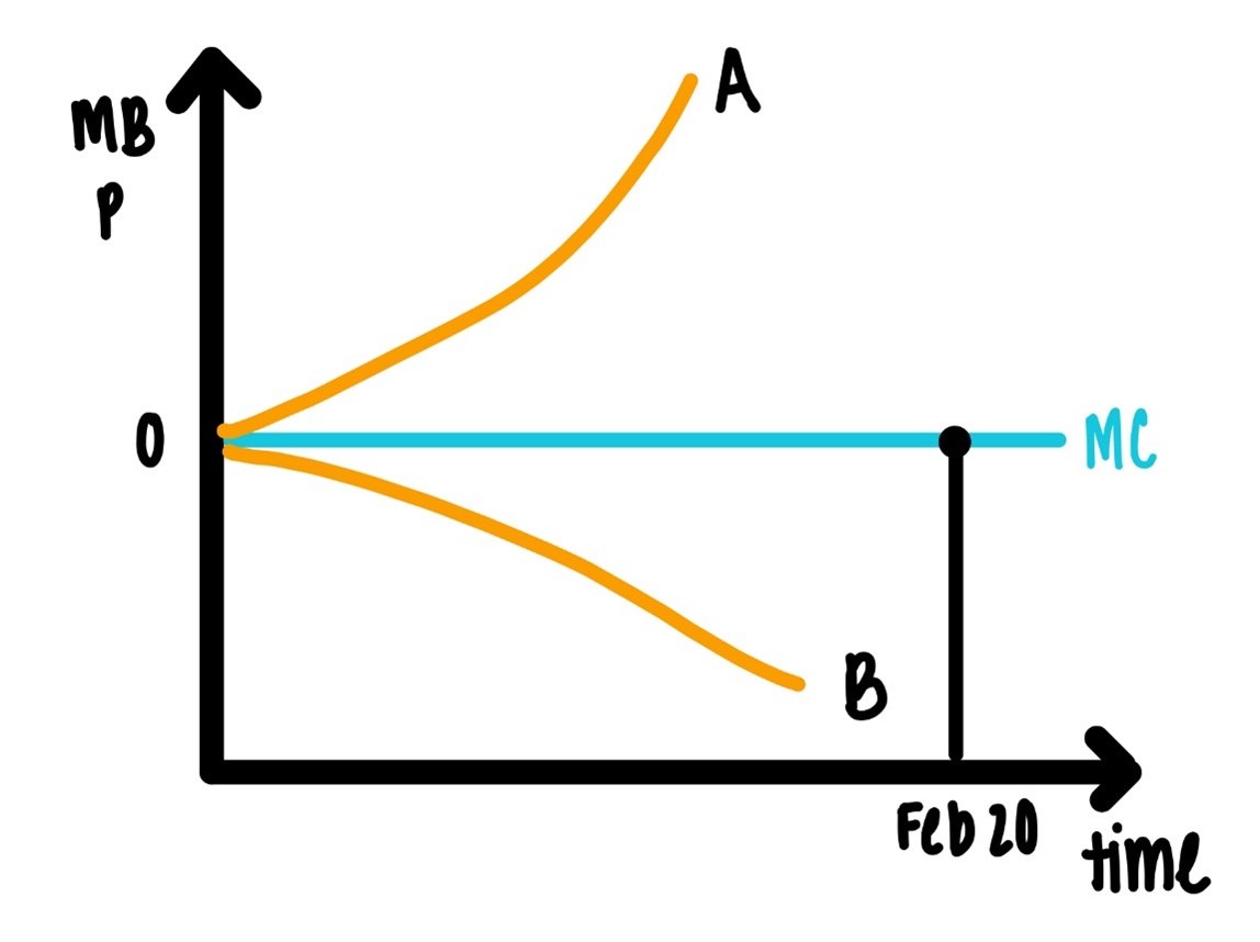
Figure 9.11: College Gameday Pricing vs Taylor Swift Pricing

In Figure 9.11, price charged by IU is constant at $\$50$. If IU has a terrific season, then the willingness to pay will rise as indicated by the curve $0A$.

If the willingness to pay rises, the profit maximizing price rises as well. The IU price does not. The IU pricing policy is not profit maximizing.

It could happen that IU has an even worse season than expected. Then Hoosier willingness to pay would drop as indicated by the curve $0B$. In that case the profit maximizing price will drop as well. The IU price does not.

The IU pricing policy is not profit maximizing.

The IU pricing policy is unusual. There are no for-profit firms that do what IU does.

You can buy a seat on an airplane to LA for February 20. That price will vary over time.

The price of a vacation resort for a vacation that starts on February 20 will vary over time.

The price of a ticket for a Taylor Swift concert on February 20 will vary over time, especially if it is announced mid-January that Arianna Grande will have a concert on February 20 in the same city.

The IU price does not vary, regardless of external conditions or the performance of the team. We can call the IU practice “static pricing” and the practice of hotels, airlines, musicians “dynamic pricing”.

What is a consequence of IU static policy?

Secondary markets, StubHub, etc.

Who benefit from these secondary markets for tickets?

StubHub
People selling tickets on StubHub
People buying tickets on StubHub

Who does not benefit from the secondary markets?

If Taylor Swift can figure out how to maximize profits, why can IU not do the same? Or is it that they can or could, but that they do not want to?

Advertising

Why do (some) companies advertise?

What is the role of advertising?

Why is advertising more prevalent in some industries than in others? I you drive between Indianapolis and Bloomington, you will see lots of billboards and other media advertising diamonds, tourist sites, legal services. You will not see advertisements for lettuce, pencils, strawberries.

What are optimal levels of advertisement?

We will start with a comparison of two industries, and we may assume, for now, that both are monopolies. Let’s call them industry I and industry II. Industry I has higher (in absolute value) elasticity of demand than industry 2.

Since monopolist 1 faces more elastic demand than monopolist 2, monopolist II will have higher mark-ups.

Which of these two firms will have a higher incentive to advertise?

If the goal of advertising is to attract more customers, to sell more stuff, the answer is clear.

The firm with the higher mark-ups has the highest incentive to advertise, since each new customer generates a higher profit. We can think of this as an example of rational action from chapter2. Advertising has a marginal cost: the extra dollar spend on advertising is the marginal cost. The marginal benefit of advertising is the extra profit generated by one extra advertising dollar. The marginal benefit curve for monopolist II is higher (everywhere) than the marginal benefit for monopolist 1. Therefore, monopolist II will have a larger advertising budget than monopolist I.

We can conclude:

The profit maximizing advertising expenditure is inversely related to the elasticity of demand.

As we stated earlier:

Know thine elasticities!

Another way to state the above conclusion is: We expect the degree of advertising done to be inversely related to how closely the market resembles a competitive market.

You will rarely see advertisements for strawberries, wheat, lettuce, peaches. But you will see lots of advertisements for diamonds,

9.8 Glossary of Terms

Deadweight loss of monopoly: The area, typically of a triangle, below demand, above marginal cost, to the right of the quantity sold.

Dynamic pricing: Setting a price for a future event that does allow for changes in the face of changing relevant information such as changes in the number of competing products or changes in consumers’ willingness to pay.

Marginal Revenue: The extra revenue obtained by selling one more unit.

Market power: The ability to raise the price above marginal cost.

Market segmentation: Dividing up a market demand into several subgroups so that each subgroup may be charged a different price with the goal of obtaining maximum profit from the entire market.

Mark-up: The ratio of price divided by marginal cost.

Monopoly: A market that has only one seller of a particular good that has few substitutes.

Perfect price discrimination: The pricing policy of charging each consumer their particular personalized price.

Profit ratio: The ratio of profit to total revenue.

Static Pricing: Setting a price for a future event that does not change even in the face of changing relevant information such as changes in the number of competing products or changes in consumers’ willingness to pay.

9.9 Practice Questions

9.9.1 Discussion

Discuss reasons why the IU Athletic Department might not want to adopt dynamic pricing.
When a cruise ship leaves the harbor with one empty cabin, that empty cabin represents lost revenue and thus lower profit for the company. When there is one empty seat at an IU football game, that also represents lost revenue for IU. Discuss a pricing policy that would increase the probability to close to one that all seats at IU football games will be sold. What are disadvantages of your proposed pricing policy?
How would you detect monopoly power in the health care market in Bloomington, IN? How would you measure it? How good are your measures?
List and discuss four factors that might influence the effectiveness of advertising.

9.9.2 Multiple Choice

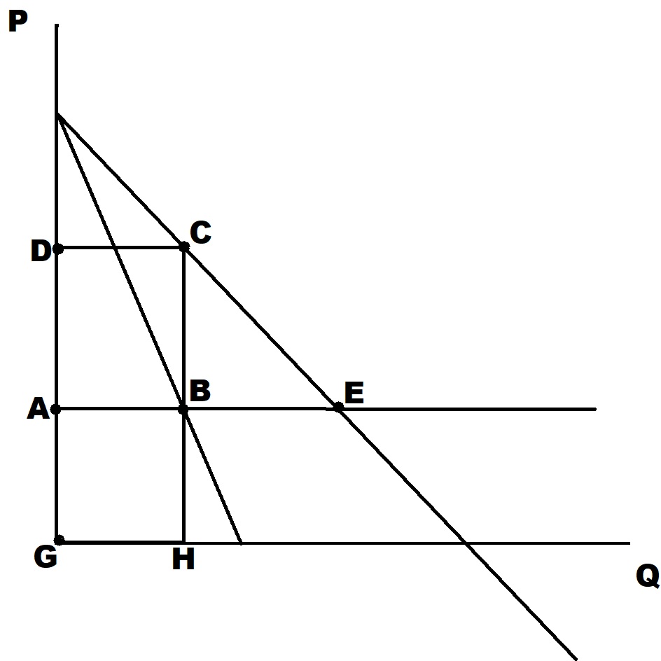
Figure 9.12: For problems 1-3.

In Figure 9.12 above the area ABCD represents

A. Total revenue for the monopolist
B. Total profit for the monopolist
C. The deadweight loss of monopoly
D. Consumers’ surplus
In Figure 9.12 above the area GHCD represents

A. Total revenue for the monopolist
B. Total profit for the monopolist
C. The deadweight loss of monopoly
D. Consumers’ surplus
Imagine that in Figure 9.12 marginal costs drops by 15%. The we would expect

A. Consumers’ surplus to increase
B. Total profit to increase
C. The price to decrease
D. All if the above
In Figure 9.12 above the most efficient point is

A. C
B. B
C. E
D. F
Imagine in Figure 9.12 above that the government imposes a price ceiling that is below the line DC. Then

A. The monopolist’s profit will decline
B. Consumers’ surplus will increase
C. The quantity sold will increase
D. All of the above
In problem 5 above, the quantity sold will increase because

A. The price ceiling becomes marginal revenue
B. The price ceiling becomes marginal cost
C. The price ceiling becomes demand
D. The price ceiling becomes total revenue
Imagine that the city of Chicago organizes a mile run down Michigan Avenue with the six best milers of the world. This race takes place in 5 months. The city closes of the area around the racecourse and charges ticket prices to attend and view this event. Imagine that the price for this event charged by the city of Chicago stays constant between now and the event. The beneficiaries of such a pricing policy are

A. Organizers of secondary ticket markets such as StubHub
B. The people who buy tickets on such secondary markets
C. The people who sell tickets on such secondary markets
D. All of the above
Image you observe the following: There are two types of people, grayhairs and brownhairs. At restaurants grayhairs typically face prices that are ten percent lower than prices for brownhairs. We can conclude that

A. Both types of consumers have equal elasticity of demand
B. Grayhairs have lower elasticity of demand than brownhairs
C. Grayhairs have higher elasticity of demand than brownhairs
D. Grayhairs have perfectly inelastic demand
A per unit subsidy to a monopolist can increase efficiency in that market because

A. The monopolist on his/her/ their own does not produce enough
B. It can lower marginal cost, and this induces the monopolist to produce more
C. It moves the intersection of marginal cost and marginal revenue to the right
D. All of the above
Segmenting the market into two segments and charging different prices in the two segments

A. Always increases profit
B. Decreases profit
C. Increases profit if it is very difficult for consumers to transfer the good from one of the segments of the market to the other
D. Decreases profit if it is very difficult for consumers to transfer the good from one of the segments of the market to the other
We would expect advertising intensity, measured by advertising expenditures relative to total revenue, to be

A. Positively correlated with the price-cost markup
B. Negatively correlated with the price-cost markup
C. Positively correlated with marginal cost
D. Positively correlated with the price
We would expect the price-cost markup to be

A. Negatively correlated with the elasticity of demand
B. Positively correlated with the elasticity of demand
C. Positively correlated with marginal cost
D. Negatively correlated with marginal cost
The fundamental difference between a monopolist and a firm in a competitive market is

A. The firm in a competitive market faces a flatter demand curve than a monopolist
B. The firm in a competitive market faces a steeper demand curve than a monopolist
C. The firm in a competitive market faces a downward sloping demand curve, while the monopolist faces a horizontal demand curve
D. The firm in a competitive market faces a horizontal demand curve, while the monopolist faces a downward sloping demand curve
For a non-price discriminating monopolist marginal revenue is

A. The price
B. Horizontal
C. Vertical
D. Below demand
For a monopolist who is engaged in perfect price discrimination the marginal revenue is

A. The consumer’s reservation price
B. Below the consumer’s reservation price
C. Above the consumer’s reservation price
D. Equal to marginal cost
Static pricing is not profit-maximizing because

A. It ignores relevant changes in demand
B. It ignores relevant changes in availability of substitutes
C. It ignores relevant changes in external conditions that influence demand
D. All of the above
Imagine that a monopolist practices perfect price discrimination. Then the level of output is

A. Efficient
B. Below the efficient level
C. Above the efficient level
D. Determined by the lowest point on the marginal cost curve
Imagine that a monopolist is practices perfect price discrimination. Then consumers’ surplus is

A. Zero
B. Negative
C. About half the size of what it would be in a competitive market
D. Bigger than what it would be in a competitive market
A monopolist can only practice market segmentation if

A. There are estimates of the demand elasticities available and if these estimates differ across segments
B. If it is very difficult to transfer the good from one segment of the market to another
C. There are no differences in transportation costs between the market segments
D. a. and b.
In a monopoly the demand curve shifts out (for whatever reason). Then we would expect

A. Consumers’ surplus to increase
B. Monopoly profit to increase
C. The price to increase
D. All of the above

8 Externalities

10 Game Theory

Q	P	TR	MR
1	\(\$9\)	\(\$9\)	\(\$9\)
2	\(\$8\)	\(\$16\)	\(\$7\)
3	\(\$7\)	\(\$21\)	\(\$5\)
4	\(\$6\)	\(\$24\)	\(\$3\)
5	\(\$5\)	\(\$25\)	\(\$1\)
6	\(\$4\)	\(\$24\)	\(-\$1\)
7	\(\$3\)	\(\$21\)	\(-\$3\)
8	\(\$2\)	\(\$16\)	\(-\$5\)