7 Competitive Markets

In this chapter we will learn:

Understand how shifts in supply and demand determine prices and quantities
Understand what factors shift supply and demand
Use the supply and demand framework to evaluate some policies
Understand the economic consequences of taxation in the competitive market framework
Understand the consequences of price ceilings like rent control
Understand the notion of an efficient allocation
Understand why competitive market allocations can be efficient

7.1 Competitive Equilibrium

We are now in a position to put together supply and demand to “make” our model of competitive markets. We think of competitive markets as markets where there are many sellers and many buyers so no individual can influence the price. Each seller and each buyer acts as a price taker.

Each seller who is a price taker faces a horizontal demand curve. At the established market price, the seller can sell as much as he/she likes, whatever is the profit maximizing amount.

This holds for the buyer as well. At the established price the buyer can purchase as much as he/she likes, whatever is the utility maximizing amount.

The market sets the price and given this price, all participants in the market make the decisions that are individually best for them. Prices will not be influenced by individual behavior.

If I decide to drink less coffee, the price of coffee in Bloomington, IN will not change. Of course, if half of the coffee drinkers give up coffee for tea, that is a different story. Such a change in coffee demand would move the price.

There are many real-world markets that can be analyzed in the framework of competitive markets. If I wanted to figure out whether a substantial change in IU enrollment has any impact on the Bloomington housing market I would start with a model of competitive markets for rental units.

In Figure 7.1 below we illustrate how competitive markets work. The supply curve is upward sloping, the demand curve is downward sloping. These two curves intersect at quantity $Q^*$ and price $p^*$. We call this point the competitive equilibrium.

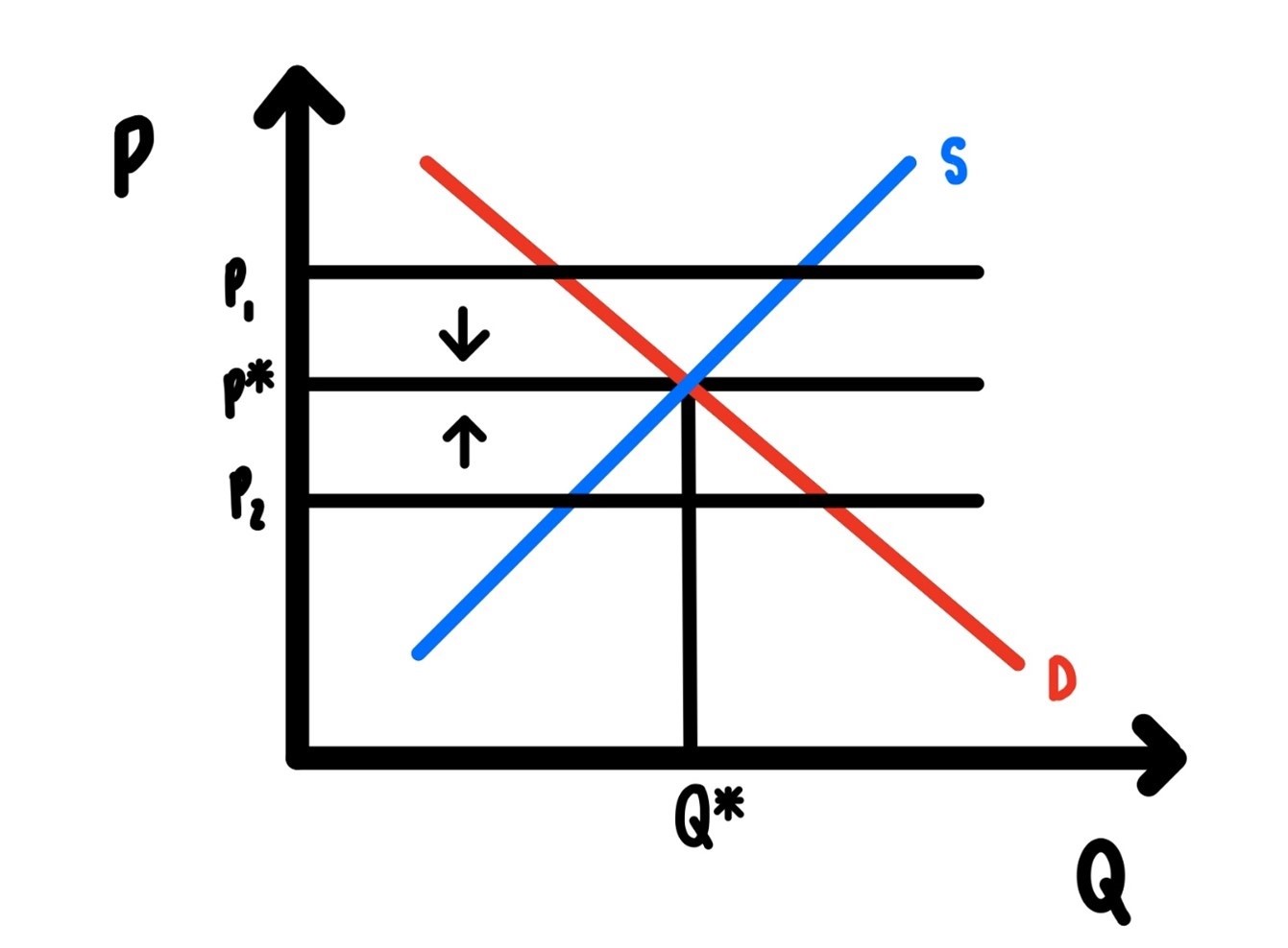
Figure 7.1: Competitive Equilibrium.

Why would this be the equilibrium and not some other point? If the price were $p_1$, the quantity supplied would exceed the quantity demanded. A large part of inventory would not be sold. The firm would be very tempted to lower the price in order to sell more inventory. There would be downward pressure on the price. Then prices would tend down toward $p^*$.

If the price were at $p_2$, then the quantity demanded is larger than the quantity supplied, i.e., we have excess demand, there would be upward pressure on the price and the price would be pushed toward p*.

At price p* the decisions by the buyers are consistent with the decisions of the sellers. This is the only price where this happens. At higher prices, firms want to sell more than households want to buy. At lower prices households want to buy more than firms are willing to sell.

7.2 Consumer/Producer Surplus

In Figure 7.2 we illustrate the concept of consumer surplus. In the figure the equilibrium price is $p$. At this point, the number of units sold is $Q$. For all customers who buy the product the marginal benefit of one more unit of the product is higher than the price. It has to be. The transaction is voluntary. No consumer would spend more than the value they attach to the product. So, whoever is buying the product, is getting more than they are paying, they are getting a surplus. That surplus from one particular unit sold is indicated by the distance of the vertical line segment $\text{KL}$. This surplus applies of course to all units sold. Adding up all the surpluses for all the goods sweeps out the entire area of the triangle $\text{ABC}$.

We call this area Consumers Surplus, or $\text{CS}$. We will use consumers surplus as one measure of welfare in the market.s

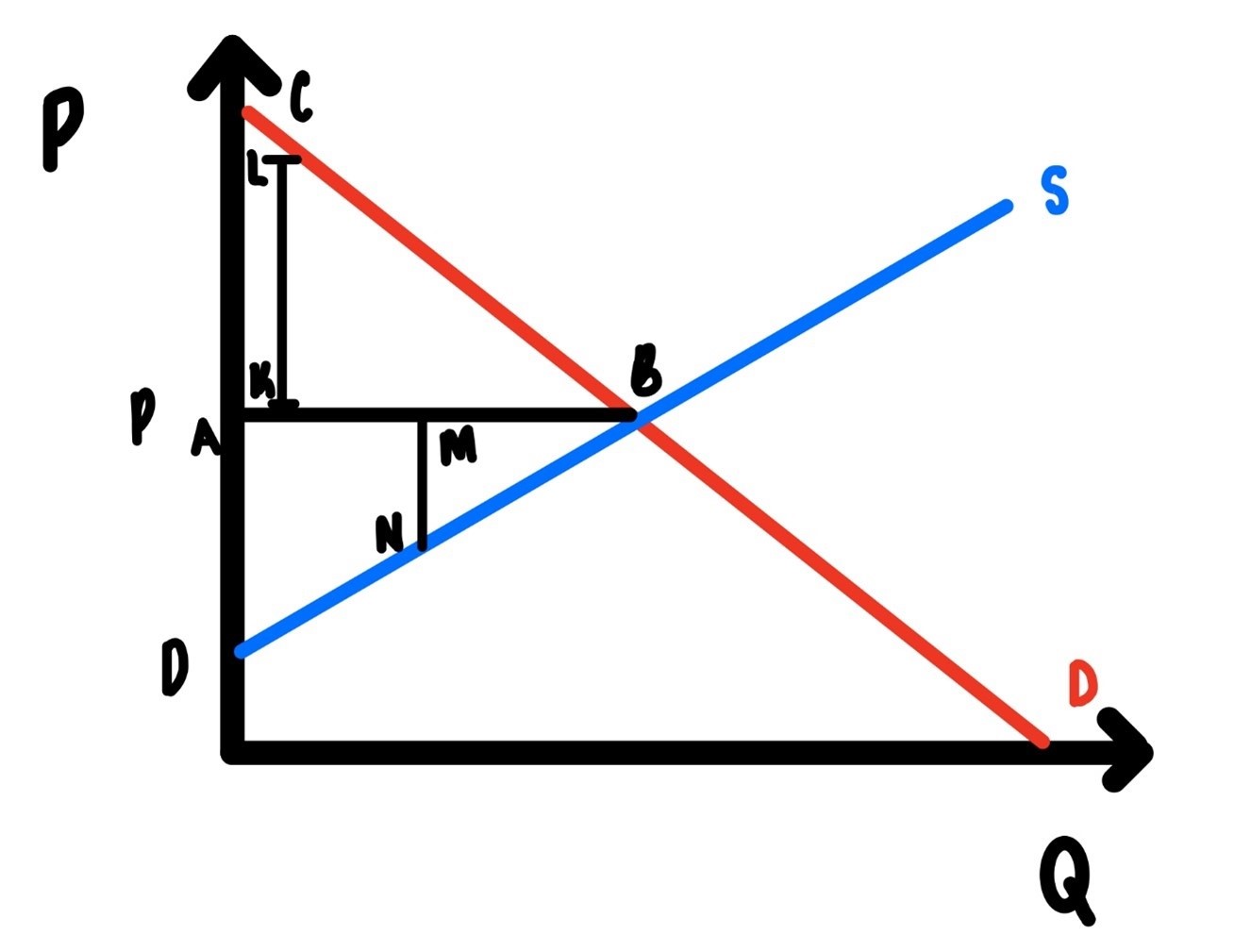
Figure 7.2: Competitive Equilibrium.

There is a similar surplus for producers. For all the units sold the marginal cost of producing is less than the price. For each one of these units, the firm is getting a surplus. This surplus is indicated by the length of the vertical line segment $\text{MN}$. Adding all these surpluses up sweeps out the triangle $\text{ADB}$.

This area is called Producers’ Surplus, or $\text{PS}$.

The sum of consumers’ surplus and producers’ surplus will be called welfare, $W$. We thus have

\[W = CS + PS\]

One of the nice things about this construct is that it allows us to evaluate economic policies. In general, policies that shrink $W$ impose a welfare loss and policies that increase $W$ generate a welfare gain. Moreover, we can assign quantitative, numeric values to welfare gains or losses from various policies.

7.3 Unit Taxation

Imagine that the government collects a tax on firms. The tax takes the following form: For each unit sold the firm has to pay $\$t$ to the government. How could this tax be incorporated into our model of the competitive market?

With the imposition of the tax, the marginal cost of the firm rises. It rises exactly by the amount of the tax, $\$t$. This is illustrated in Figure 7.3.

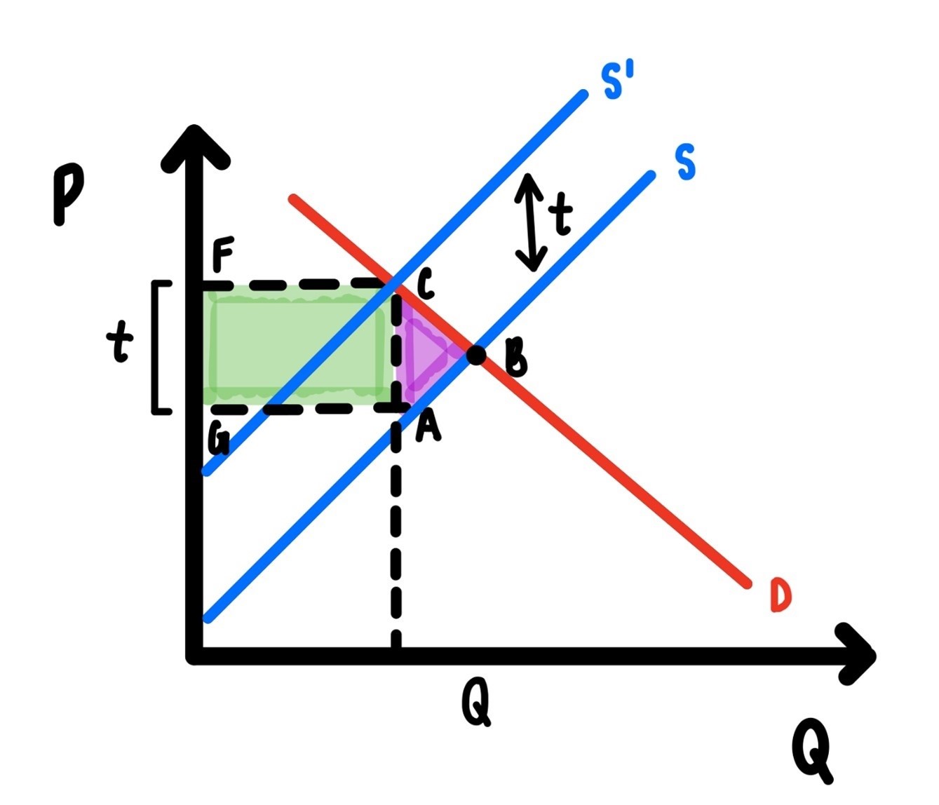
Figure 7.3: Unit Taxation.

In Figure 7.3, the usual supply and demand curves without the tax are labelled $S$ and $D$ as in the previous figures. With the imposition of the tax, the marginal cost shifts up by $\$t$. Since supply is marginal cost, supply shifts up (or to the left), by the amount $\$t$. This new supply curve is labelled $S’$.

The equilibrium is now at point $C$ with quantity $Q_t$ and price $p_t$. Without the tax, the equilibrium would have been at point $B$. We can use this to answer some questions.

How big is the tax revenue collected?
What happens to consumers’ surplus because of the tax?
What happens to producers’ surplus?
How much value is lost through taxation?
The tax on each unit is $t$. The total quantity sold is $Q$. Thus, the tax revenue is $tQ$. This is indicated by the area of the rectangle $\text{GACF}$.
Due to the tax, the price rises and the quantity falls. This means consumers’ surplus must decrease.
The same as to consumers’ surplus. The price drops and the quantity sold falls. So, producers’ surplus has to fall as well.
Another way of asking is what is the area of the triangle $\text{ABC}$? That is the deadweight loss of taxation. This area is measure of the welfare or efficiency loss incurred through taxation. If you go just one unit beyond $Q$, some consumer would be willing to pay more than the marginal cost of producing that unit. At that point demand $D$ is higher than supply $S$. Surely, efficiency requires a trade to take place when the willingness to pay for one more unit is higher than the marginal cost. Because of taxation, potentially welfare-improving trades do not happen. That is why the area ABC is called the deadweight loss of taxation.

Note: Just because taxation imposes a deadweight loss does not imply that taxes are bad. We must always compare the size of the deadweight loss incurred through taxation with the benefit that is possible only through the programs/expenditures the government can finance only through taxation. These include such things as expenditures on national defense, the justice system, the EPA, FDA, expenditures on COVID-19 testing, etc. For some of these the gains from the program/expenditure might exceed the deadweight loss of taxation, but not for others. Whether program benefits exceed the deadweight loss of taxation depends on a carefully done cost benefit analysis.

7.4 Price Ceilings

Often governments decide that prevailing prices are too high. Then they impose price ceilings. Prominent examples of this are rent control and anti-price gouging laws. We will consider these in turn.

Figure 7.4 illustrates the effect of a price ceiling like rent control. The demand and supply curves are designated $D$ and $S$, respectively and the equilibrium price is $p$. Imagine that the government imposes a price ceiling of $p’$. For the price ceiling to be effective, it has to be binding, i.e., be below $p$.

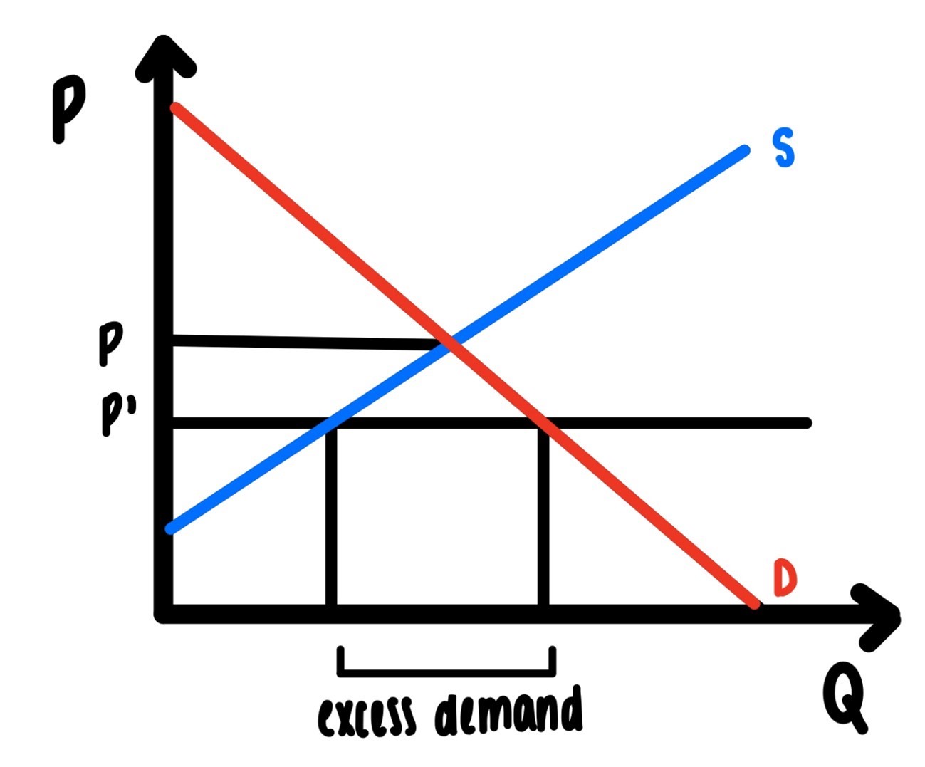
Figure 7.4: Unit Taxation.

LOOK A BIT LIKE THE FIRST PANEL FROM RATIONAL CHOICE CHAPTER?

At the price $p’$ the quantity supplied is below the quantity demanded. There is excess demand.

People who would like to get an apartment at the price $p’$ cannot find one. Immediate consequences are homelessness, couch surfing and doubling up. So, who benefits and who loses from rent control? The obvious losers from rent control are those people who cannot find a place. The beneficiaries are those who get to stay in their apartments with lower rents.

But there is more. Other consequences are:

Commuting distances will increase. If, for example, Bloomington, IN passes a rent control law for the city of Bloomington, many IU students would probably find apartment in outlying communities such as Ellettsville.
The quality of apartments goes down. As the rent drops, landlords will not have the funds and/or the incentives to maintain the apartments. It is then not clear whether those renters who stay in rent-controlled apartments will really benefit.
Turnover will probably drop. Those tenants who are lucky enough to be in a rent-controlled apartment and who do mind the lack of maintenance will tend to stay longer than without rent control.
Key money. For rent controlled apartments one often finds other under the table side payments. The rent control will fix the monthly rent, but if it does not specify a payment for the apartment key, there will be a temptation for the landlord to ask for “key money”. The rent will be at the prescribed level, but the key might cost $\$500$. There may be other side payments as well. This comes under the category: If the government imposes rules that are contrary to the interest of some people, some people will do what they can to get around the rules.
Apartments are more likely to be turned into condominiums. Condominiums are typically not covered by any rent control legislation and their prices are typically set at higher levels by the market.

7.5 Examples

Example 1: Beef vs Chicken

In the last 20th century, we saw Americans buying less beef and more chicken. The big question is why? Most people would attribute this change to a shift in demand. The story goes like this: At the time people realized the unhealthy consequences of eating (too much) red meat and they switched to chicken. One way to think about this explanation is: the demand for beef decreased and the demand for chicken increased.

If this is true, then we would have seen an increase in the price of chicken relative to beef. This is illustrated in Figure 7.5. A decrease in beef demand and an increase in chicken demand lowers the price of beef and increases the price of chicken. This is indicated by the arrows labelled 1 in the graph.

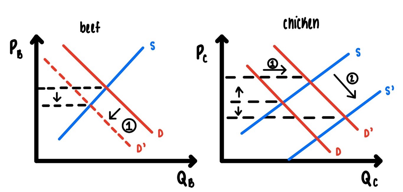
Figure 7.5: Unit Taxation.

This story sounds eminently plausible. There is only one problem with this story, this theory. At that time the price of chicken relative to beef dropped. How could that be explained? This drop in the price of chicken cannot be explained by the shift in demand away from beef to chicken. That goes in the wrong direction. The other possible explanation is that there was massive technological progress that shifted the marginal cost of chicken production way down, as illustrated by the arrow labelled 2 in the figure. That is not to say that the demand shift did not happen. It just says, since the price of chicken relative to beef dropped, the shift in supply (marginal cost) must have been bigger than the shift in demand, the health concern.

Example 2: A Tool to Fight Recessions

Imagine that now, in the middle of the COVID-19 induced recession, the government made the following announcement: Starting January 1, 2024, we will raise a luxury tax on all yachts. The tax rate will be 80%. How would markets respond to this announcement?

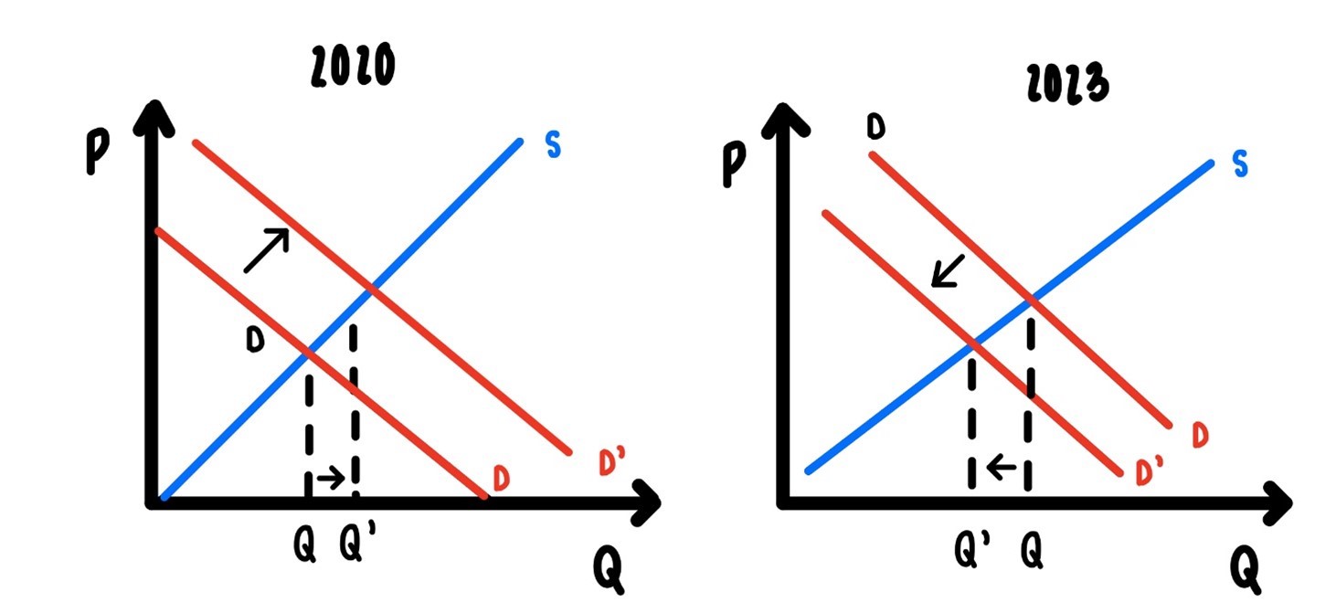
Figure 7.6: Unit Taxation.

Many wealthy people who are considering purchasing a yacht might say: Instead of waiting three years for the yacht, I will buy it now. Yachts are durable goods and a yacht in three years is a decent substitute for a yacht now, and vice versa. As the price of the yacht in three years rises, demand for yachts today will increase. If demand today increases, the price of yachts today increases, and the quantity of yachts traded/sold today will increase. See Figure 7.6.

Why is this a recession fighting tool? Well, if you want to sell more yachts, you must produce more and if you want to produce more yachts you need more labor, more capital, more material inputs. That is exactly what we want to do and accomplish in a recession.

Of course, this does not only apply to yachts. It also applies to private jets, expensive diamonds, and all other luxury goods that are purchased by the wealthy.

Example 3: A Green Paradox

Many policies that are proposed in this country to combat global climate change are policies that shift demand for fossil fuel to the left, i.e., decrease demand for fossil fuel. As illustrated in Figure 7.7, panel a, that decrease in demand, if the policies are successful, will decrease the price of fossil fuels.

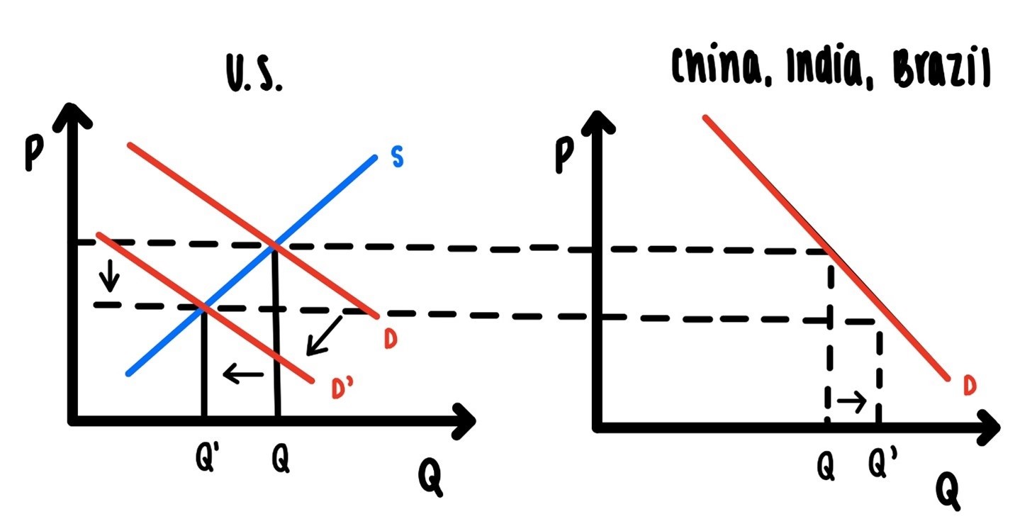
Figure 7.7: Unit Taxation.

But that is not the end of story. Fossil fuels are traded on a world market. If a large economy like the US economy reduces its demand for fossil fuels massively, there is likely a massive reduction in the world price. If there is a large reduction in the world price of fossil fuels, other countries like China, India, Brazil will just walk down their downward sloping demand curve and consume more fossil fuels. Punchline: The US policy of reducing US demand for fossil fuels is like to do very little to decrease the GLOBAL output of $CO_2$ and equivalent gases.

Example 4: Another Green Paradox⁴²

We have heard it time and time again. By the year 2050 we will reduce demand for fossil fuels by something like 40 or 50%, by a large fraction in any case. Good intention/policy or bad intention/policy?

Some simple economics comes into play. See Figure 7.8.

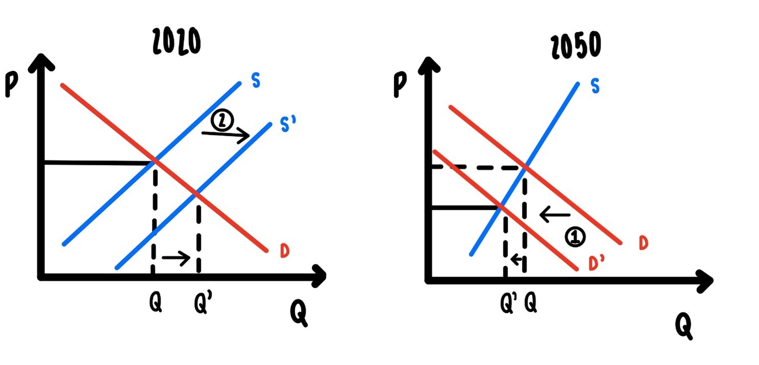
Figure 7.8: Unit Taxation.

A large reduction in the demand for fossil fuels in the year 2050 will lower the price of fossil fuels in the year 2050. So, the Saudi Oil Minister can either sell a barrel of oil today at $\$40$ or, he can expect to sell the barrel in 30 years at a lower price, say $\$30$ per barrel. If you are the Saudi Oil Minister, would you rather sell at $40 today or at $\$30$ in the future? You would rather sell today.

In this case oil extraction will be shifted from the future to the present, i.e., the oil supply in 2050 will shift left (decrease) and the oil supply today will increase (shift right).

As oil supply today increases, the price will drop and people will drive more, buy more fuel inefficient cars, have bigger homes, choose longer commuting distances, etc.

All of this will increase current $CO_2$ output in the present. Which, I think, is the last thing we would want.

At this state you may say that this is just theory, that this is just “academic” in the often-derogatory common use of that term, that this has nothing to do with the real word. Unfortunately, this is not so. There is some evidence from natural resource economics that announcements of future policies will have current effects and these effects that we find in the data are just what the theory predicts. The evidence comes from the Clean Air Acts Amendments from 1990 and the Acid Rain Program from 1995. The Acid Rain Program put limits on sulfur-dioxide emissions and made it clear that it would be difficult to sell coal in the future. How did coal markets respond to this announcement?

First: The supply of coal increased immediately, causing an immediate drop of the price of coal of 9%.

Second: We would expect this effect to be biggest for sulfur rich coal. It was. The supply of sulfur rich coal increased more than the supply of “normal” coal. Therefore, the price of sulfur rich coal dropped more than the price of “normal” coal. Since high sulfur coal sells at a discount, the sulfur discount increased substantially. By 40%. That is big!

Example 5: Tariffs on China

The Trump administration imposed a 25% tariff on Chinese textiles. This was with the hope of giving the American textile industry a shot in the arm and reviving the American textile industry. Figure 7.9 below shows the effects of the tariff.

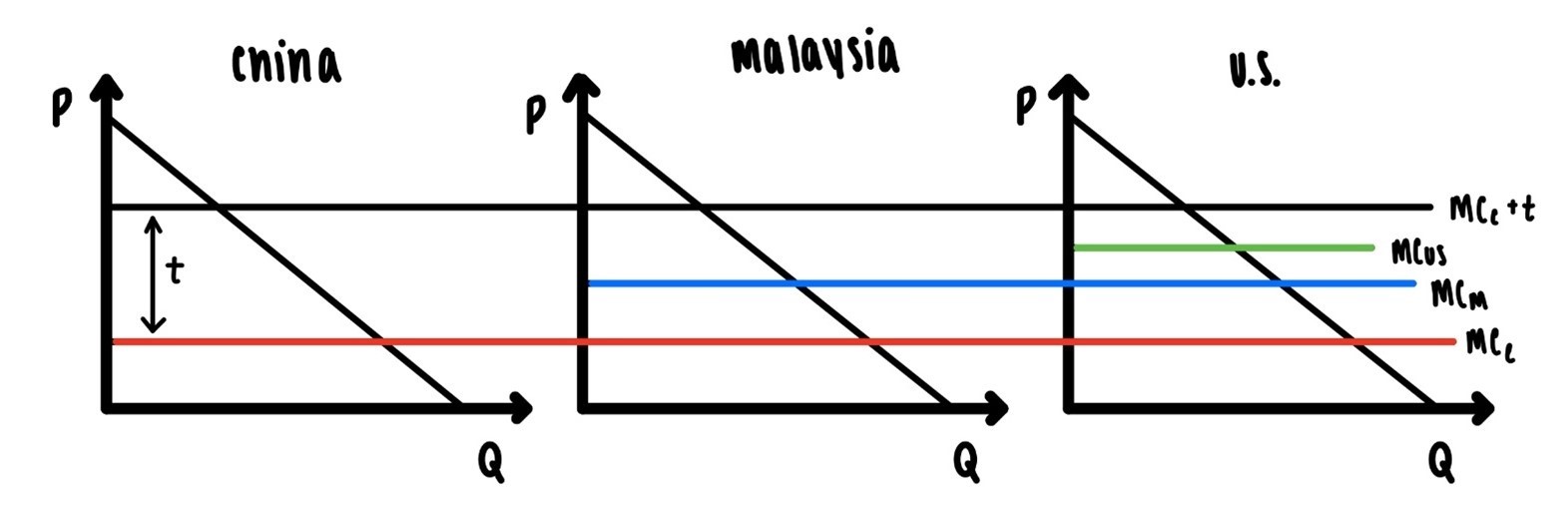
Figure 7.9: Unit Taxation.

The imposition of the tariff increased marginal cost in China to a level perhaps higher than US marginal cost. This must be so if there is any hope to revive this industry in the US. If the tariff did not increase Chinese costs above US levels, why would cost minimizing firms incur these high costs in the US?

But there is one issue that matters. There are other countries with vibrant textile industries: Vietnam, Thailand, Bangladesh, Malaysia just to name a few. In those countries marginal cost of production, adjusted for quality, must be higher than in China, otherwise these countries would be the major importers into the US. This is illustrated in Figure 7.9, where the marginal costs are higher in Malaysia than in China, before the tariff. Figure 9 also shows that marginal costs in China after the tariff are higher than in US.

How does the tariff impact textile industries in these three countries?

China’s textile industry will shrink.
The textile industry in Malaysia will grow, since there will be a shift from China to Malaysia.
There will be minimal impact on the textile industry in the US, since Malaysia is a cheaper producer.
Textile prices in the US will rise and the standard of living fall, since the tariff induces firms to switch from a very low-cost international supplier to another international supplier, whose costs are higher.

Example 6: Who Pays for Tariffs?⁴³

Who pays for the tariffs on Chinese imports imposed in 2017 and 2018, importers or exporters? Firms or consumers?

In 2018, the Trump administration-imposed tariffs on many goods such as washing machines, solar panels, steel, aluminum imported from several countries and on several hundred billion worth of goods imported from China. This happened in waves in July 2018, August 2018, and September 2018. The rates were 10% or 25% depending on the good. In May 2019 the 10% rate was increased to 25% on many goods. China and many other countries responded by imposing tariffs on their own imports from the US.

We want to know how prices responded, both in the case of prices of imports and in the case of prices of exports.

There are many possibilities. Imagine a market for washing machines with a large number of firms and that some of these washing machines are imported from China. The firms that are hit with the tariffs, foreign firms, now face a higher marginal cost and the domestic firms have a cost advantage. Will the “domestic market” respond by increasing prices to the higher level that might be implied by the tariffs? Or will the foreign market respond by decreasing pre-tariff prices to be still competitive with the firms in the “domestic market”? Both of these are reasonable consequences. Which of these will happen or in which combination is an open question. Cavalo et al. (2021)⁴⁴ addresses exactly these issues.

But what prices? You may think this is a stupid question, but there is really something to it. An imported washing machine, say, has a price as it crosses the border. That price is not necessarily the same when that washing machine is sold at your favorite store in Indianapolis. The border prices are collected through the International Pricing Program of the Bureau of Labor Statistics. For the prices at retails stores the authors use data from 30 large retail stores. These prices are scraped daily from the stores’ webpages. The estimates are done at the product category, i.e., each data point is a product i imported from country j in sector k in month m. There are lots and lots of data point, over 800,000, so things can be estimated rather precisely.

Here are two results from this estimation:

For imports into the US, a 10% increase in the tariff leads to a reduction in the pre-tariff price at the border of less than 0.6%. That is very small.
For exports from the US to other countries, a 10% increase in the (retaliatory) tariff is associated with a reduction in the pre-tariff price at the border of 3.3%. That is more than 5 times bigger than the effect of tariffs on the goods imported into the US.

Why? On the face of it, this large difference makes no sense.

What we have is a situation where country 1 imports from country 2 and country 2 imports from country 1. Each country imposes a tax/tariff on the gods it imports from the other country. This sounds like a perfectly symmetrical situation and therefore, the price effect of the tariffs ought to be at least roughly equal and not differ by a factor of five or six.

So, what on earth is going on?

The authors distinguish two types of goods: differentiated goods and undifferentiated goods. Differentiated goods are things like microwaves, bicycles, chain saws, coffee makers, drones, etc. Undifferentiated goods are things like wheat, soybeans pork, lumber, etc. One way to think about this distinction is: for differentiated products branding matters, but not for undifferentiated products.

What the paper finds is:

For differentiated products the tariff effect on prices is indistinguishable from zero.
For undifferentiated products, the tariff effect is negative and large.

So how can we reconcile results 1 and 2? Well, the US exports predominantly undifferentiated products and imports mostly differentiated products. Therefore, for US export, the effects of the from the undifferentiated products dominate the effects from the dominates the effect of the differentiated products.

Example 7: The China Syndrome

The paper linked here, documents that between 1990 and 2007 imports from China into the US destroyed 1.5 jobs in manufacturing. Big effect? Small effect? How would you determine?

This paper https://economics.mit.edu/files/11606 shows that large losses in income for some American workers associated with Chinese import penetration. In fact, US manufacturing workers at the 75th percentile of trade exposure to Chinese imports experience income over the long haul that is 46% lower than income of those workers who are at the 25th percentile of trade exposure. Larger exposure to Chinese imports lowers income. That effect is large.

Economic theory predicts that such large labor market effects must have some implications for prices. In fact, we would expect prices of consumer goods to drop, in response to Chines import penetration.

This effect is estimated here: https://pubs.aeaweb.org/doi/pdf/10.1257/aeri.20180358 . Using data from the Nielsen Homescan Panel, which has very detailed information on prices of individual products, such as 12 pound bag of Kingsford Charcoal and many others, over the period from 2004 to 2015, these researchers document

The share of American household expenditures on domestically produced goods dropped substantially in response Chinese import growth. Of course, when you make this assessment and when you try to estimate the magnitude of this effect you have to be very careful about REVERSE CAUSALITY. It is not surprising that an increase in Chinese imports to the US leads to a decline in the fraction of US household expenditures going to US goods. But causality can go the other way too: A decline in US production of manufacturing goods may present itself as a profit opportunity to Chinese manufacturers, who then may decide to go in for the kill, so to speak.
A decline in the share of US household expenditures going to domestically produced goods is associated with smaller goods inflation, i.e., prices of goods rise more slowly. We might want to know how BIG is this effect. Prices of goods with median exposure to Chinese imports grow 0.17 percentage points slower than prices of goods with no exposure to Chinese imports. To get a sense of the magnitude of this effect, If prices grow at 3% annually for 10 years, after ten years they will have increased by 34 percent. If prices had grown by 0.17% less each year for 10 years, due to competition from Chinese imports, after ten years prices would be 14% higher. A whopping 20% difference!

Example 8: The China Syndrome: Horizontally we Fall, Vertically we Stand⁴⁵

Paper below distinguishes two cases. In case 1, Chinese socks compete with French socks. We call this horizontal competition. In case 2, the French use a Chinese import as an intermediate good to produce something else. In case 1 we can think of women’s jackets as the good. If there are more jackets imported from China, then we can capture this with a shift to the right of supply. This rightward shift will decrease the price, sales and employment of domestic jackets. This is exactly what the paper below finds.

On the other hand, some Chinese imports are intermediate goods in some other production process. In that case, an increase in Chinese imports, decreases marginal costs of final goods production, which can show up as an increase in sales and in employment. In the paper below, some of these effects are indeed positive but some are indistinguishable from zero.

7.6 Taking Price as given

The market determines the price, and the firm takes the price as given.

Panel a in the upper left illustrates how the market determines the price. It is exactly the price where supply and demand intersect. This is the market determined price that each household and each firm takes as given. In the upper right panel, we show how, given that price, each profit maximizing firm decides how much to produce. There is nothing new in this figure. The upper left is just the first figure from this chapter and the upper right is just the profit maximizing figure from the supply chapter.

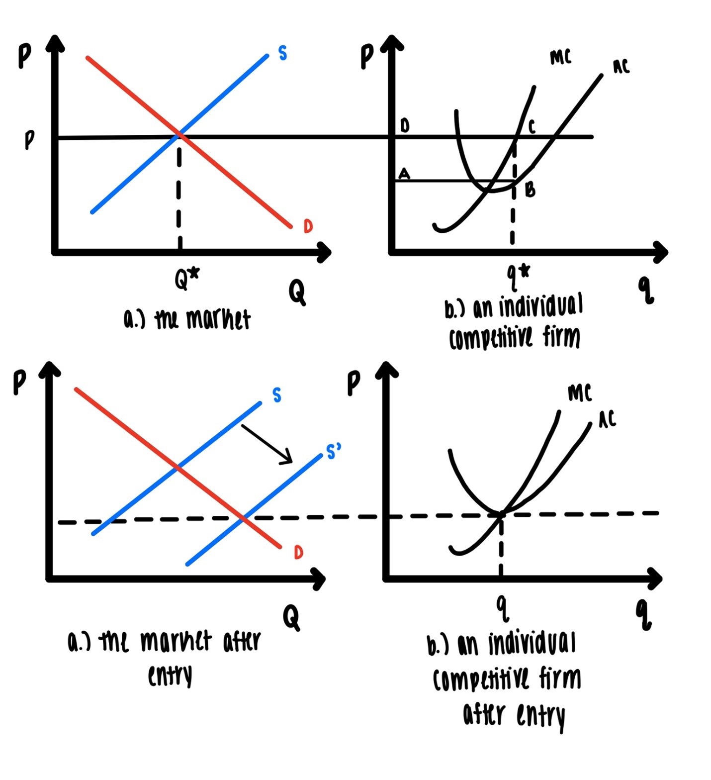
Figure 7.10: Unit Taxation.

The upper right-hand panel show the profit of the firm. At $q^*$ the average cost is given by the vertical distance from $q^*$ to $B$. The average revenue is given by the price. On each unit the firm makes a profit equal to the distance $\text{BC}$. The firm sells $q^*$ units. So total profit is given by the area of the rectangle $\text{ABCD}$.

The way the picture is drawn this firm makes a positive profit. What will happen? Other entrepreneurs will see that there are positive profits to be had/earned in this industry. This is economic profit, not accounting profit. They will enter to get a share of that pie. As they enter the supply curve shifts to the right. As the supply curve shifts to the right, the price drops.

How low can the price drop? The price can drop so that it is equal to the minimum of average costs. If it were to drop lower, it would not cover average costs, firms would make a loss and some firms would leave. As they leave, the price would rise.

So, we conclude entry and exit will move the price so that it is equal to or at least very close to minimum average costs. This is illustrated in the bottom two panels of the figure above.

At that point the firms in the industry will make zero economic profit.

Zero profit?

Yes, not zero accounting profit, but zero economic profit.

What is the difference?

Economic costs include opportunity costs. So, if you are running a ballet school, your costs of running the ballet school included the profit you could have made from your second-best alternative. Say you second best alternative is running a burger joint. Your third best option might have been working HR for a large corporation.

Your (marginal) costs of running the ballet school include the profit you could have made from running the burger joint. So, if revenue is bigger than costs, including the opportunity costs, you are making a positive profit, you are making more money running the ballet school than the burger joint. If revenue is equal to the costs, including the opportunity costs, you are making zero profit and you are making as much money running the ballet school as running the burger joint.

So, so long as your profit, your economic profit, is not negative you are doing better or at least as well, running your ballet school rather than the burger joint. If your economic profit is zero, that means that you are doing as well in your first best option, the ballet school, as in your second-best option, the burger joint. There is nothing you can do to do better financially.

The top panels would be the short run equilibrium in a competitive market and the bottom two panels would illustrate the long run equilibrium in the market.

Most textbooks would stop here with this picture. This picture in a sense is very static. There IS demand and there IS supply and there IS the price, etc. That is not how the world works. There is lots and lots of churning. In many industries or markets business come and go. There is often very little stability in the supply and the demand conditions. Typically, we would expect demand and supply to shift up or down, sometimes randomly. These movement can have all kinds of causes: changes in demand, changes in the number of firms in the industry, disruptions in the supply chain, workers demanding raises, new unexpected regulations, etc.

The long run equilibrium is a bit of a knife edge, like a cliff. One can get very close to the edge and be ok and survive in that industry. But a slight disturbance could easily push you over the cliff. As demand drops, or as marginal costs rise, the firm, if it is in a long run equilibrium, might easily be pushed over the cliff into negative profits.

Then the worry begins:

Can you make payroll?
Can you pay back the loan?
What will you do with all the equipment?
How will you pay for your children’s college tuition?
What will you do to pay your bills?
Should you start new business? How to get the startup capital?
Should you seek employment? You lost your business in a recession. The unemployment rate is 7%. How will you find a job? How quickly?

This is the stuff of sleepless nights. This is the dark side of competitive equilibrium.

7.7 Positive vs Normative Economics

Before we tackle the issue of efficiency, we need to clarify a few things.

There is a distinction between positive and normative economics.

Positive economics does two things: It describes data, and it explains data without any value judgement.

Some examples might be:

Dutch women are tall.
The unemployment rate is 8.4%.
600,000 people have died from COVID-19.

One explanation for the high unemployment rate might be that customers are afraid of becoming infected, they are staying away from restaurants, massage therapists, airplane flights, hotels, etc. and, as a consequence, many workers have been laid off.

No judgement, no evaluation. It is what it is.

Normative economics evaluates. It asks whether allocations, what people get, are good, bad, ugly, desirable, non-desirable, etc. We will always do this through the lens of efficiency.

7.8 Efficiency

We can now, finally, address the question of how efficient markets might be. We need to be clear about what we mean by efficiency. The figure below, which we have seen before many times, will help.

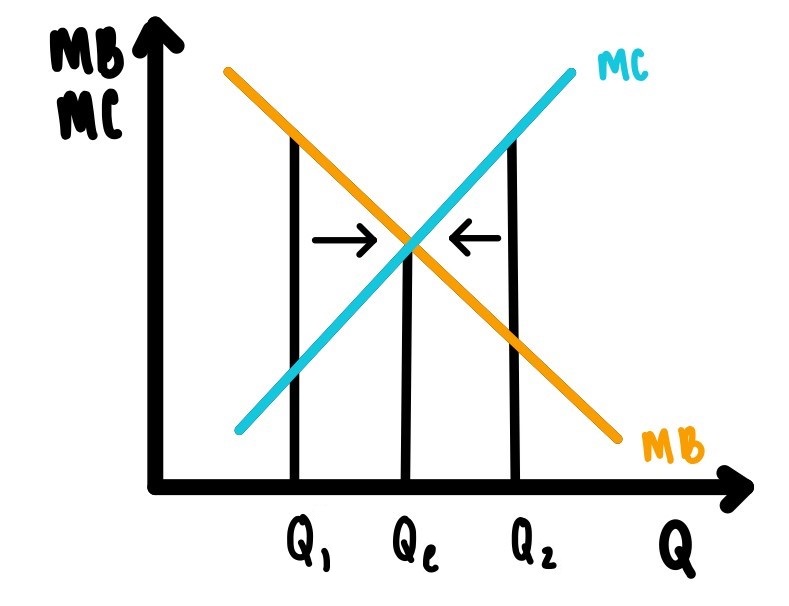
Figure 7.11: Unit Taxation.

The marginal benefit, $MB$, from beer, for example, is downward sloping and the marginal cost, $MC$, of bringing beer to the market is upward sloping. Beer is measured in six packs.

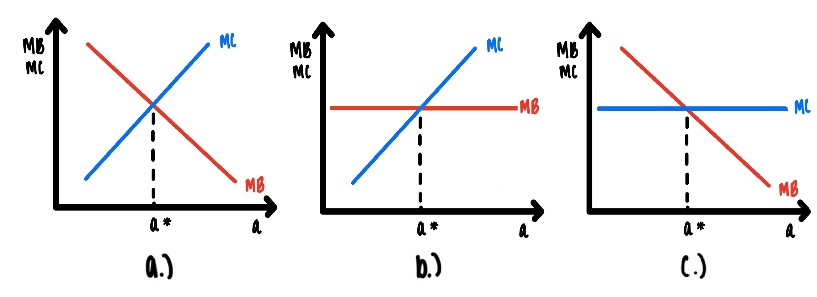
The claim is that the quantity $Q_e$, where $MB = MC$, is the efficient allocation. Why is that?

Suppose we only produced $Q_1 < Q_e$. There, $MB > MC$. The marginal benefit that some consumer gets from an extra sixpack is $\$18$, but it only costs $\$4$. That means an extra benefit could be obtained by producing one extra six pack. This extra benefit, the net benefit, marginal benefit minus marginal cost, from one more sixpack is $\$14$. And more beer should be produced, as indicated by the arrow pointing right.

Suppose we are producing $Q_2 > Q_e$. At that point, $MC > MB$. That last sixpack that is produced costs $\$20$ and it generates only a benefit of $\$5$. Producing this last unit generates a net loss of $\$15$. That last unit should not be produced. Less beer should be produced, as indicated by the arrow pointing left.

At $Q_e$, $MB = MC$. That is the efficient point. All the other points are inefficient.

There is one more slightly different, but related way of looking at this. Suppose we are producing $Q_1$. Then there is something we can do to make at least one person better off without making anyone worse off. We can produce one more sixpack. That net benefit could make at least one person better off, with an extra six pack, without making anyone else worse, if the producer of the six pack is compensated for the extra costs.

This leads to the following general definition of an efficient allocation: An allocation is efficient, if there is no other feasible allocation that makes at least one person better off, without making anyone else worse off.

Examples:

Suppose Jane and Janice have $100 bucks between them. Jane has 36 and Janice has 64. While that allocation may or may not be fair, it is definitely efficient. If I want to give Jane more, it has to come from Janice, which would make her worse off. The allocation 87 and 13 is also efficient, since in order to many one of the players better off, we have to take it away from the other, which would make her worse off.
There is a collection of 100 people, with 50 AWO and with 50 OWA. The AWOs have apples want oranges, the OWAs have apples want oranges. That allocation is not efficient. EVERYONE could be made better off. The AWOs trade their apples for oranges, the OWAs trade their oranges for apples. EVERYONE is better off.
There are two types of workers, Bs and Ws. The Bs typically live in a region called S, the Ws typically live in a region called N. The Bs discover that wages in N are 50% higher than in S. The governments in N decide to prevent the expected immigration by imposing barriers like zoning restrictions that make immigration and successful settling down in N more difficult. Without these barriers the wages would be equalized. With the barriers, wages in N will remain higher by 25% than in S. Are these barriers efficient?

We can now state the following

Fundamental Theorem of Welfare Economics: Under certain conditions, which we will have to specify and make explicit, the competitive equilibrium is efficient.

How do we know this? Let’s compare Figures 7.1 and 7.11. They are exactly the same. The demand curve in Figure IS the marginal benefit curve in Figure 7.11. The supply curve in Figure 7.1 IS exactly the marginal benefit curve in Figure 7.11. It follows that $Q^* = Q_e$, which just says that the equilibrium allocation is the same as the efficient allocation. Done.

At this point we may invoke the often-cited quote from Adam Smith, An Inquiry into the Nature & Causes of the Wealth of Nations, Vol. 1, 1777.

“It is not from the benevolence of the butcher, the brewer, or the baker that we expect our dinner, but from their regard to their own self-interest. We address ourselves not to their humanity but to their self-love, and never talk to them of our own necessities, but of their advantages.”

This quote is often used (by some) to argue against government regulation, to leave markets alone and unfettered. Of course, the theorem above only says that competitive markets are efficient. It does not say that all markets are efficient. And, the theorem states, that competitive markets are efficient only under certain conditions. We will spend a fair amount of time on studying these conditions, what these conditions are, how the violation of these conditions prevents efficiency and how frequently violations of these conditions occur. We will find that these conditions are very frequently violated and that the case for markets being typically efficient is not that clear cut.

7.9 A Macro Connection

Over the last 70 years the US economy has experienced a large decline in the manufacturing sector relative to the rest of the economy. Whether we measure the share of the manufacturing sector by employment or by value added as fraction of GDP. Between 1948 and 2016 employment in manufacturing fell from 35% of total employment down to 10%. In terms of manufacturing’s share of GDP there is a similarly large drop from 30% to 13%.

No matter how we cut, there is a large and steady drop.

This dramatic shift has profound implications for the macro economy, in particular for economic growth. More precisely: This shift implies that future economic growth cannot be as high as economic growth on the past. We will be able to understand this connection, at least a good part of it, with only a basic understanding of how competitive markets work.

We start with the insight that production processes are more amenable to technological improvements than production processes in the service sector. In manufacturing there is always tinkering to lower production costs, to make things cheaper. That is one of the consequences of competition. You got to stay ahead!

We start with a description of the production function in manufacturing, or the goods sector. The subscript $g$ stands for “goods sector”. Here $h_g$, $y_g$, $A_g$ stand for, in order, employment, measured by total hours employed in that sector, output and total factor productivity and $f( )$ stand for any production function. In order to allow for diminishing returns we assume the production function is concave.

$y_g = A_g f(h_g)$

In the service sector, we assume the following production function. In this production function the symbols have the obvious meaning. This production function is linear to express constant returns to scale. Why constant returns two scale? If a haircut takes 20 minutes, then three haircuts take 60 minutes and 5 haircuts take 100 minutes. If a meeting with a financial planner takes one hour, then three meetings take three hours and 7 meetings take 7 hours. That sounds like constant returns to scale.

\[y_s = A_s h_s\]

So, these are the two production functions in the two sectors. The fundamental difference between the two sectors that we will use here is the following: There is rapid technological progress in the goods sector and there is slow, if any, technological progress in the service sector. Using our symbols from the two production functions, Ag grows, relatively rapidly over time, while As grows slowly, if at all, over time. As Ag grows over time, marginal cost declines. Since marginal cost IS the supply curve, the supply curve in goods production falls over time. There is no such downward shift in supply in services. This is illustrated in Figure 7.12 below. That figure also illustrates how the price will drop in the goods sector, but not in the service sector.

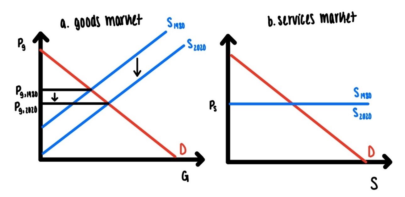
Figure 7.12: Baumols Disease

But wait, there is more.

The US economy has experienced steady growth of real per capita income, of course with some drops and fluctuations over the business cycle. The long run growth, say averages over decades has been positive. So, if we were to compare income in 2020 to income in 1980, for example, we would see vastly higher income, on average, now than 40 years ago.

We see,…

Whenever you read/hear a statement that starts with “We see……” we are talking about data, measurement, not theory. OK?

We see that the income elasticity for goods is smaller than one and the income elasticity for services is typically bigger than one. Just because your income doubles does not mean that the size of your house doubles. Elon Musk’s house is not ten thousand times bigger than mine. That income elasticity of house size measured in square feet is less than one, much less. Perhaps he has more expensive art hanging on his walls than I do.

We also see that the income elasticity for services is bigger than one. What is the evidence for that? Macro- evidence: As per capita income in the US has grown, the manufacturing sector has shrunk and the service sector has grown, both of course, relative to each other. Micro evidence: The typical family now consumes more services than a typical family 50 years ago. Just think of how many families 50 years ago would have consulted a financial planner. Also think: How many Americans got tattoos 50 years ago vs now? Moreover: as we get richer, we value the quality of services more: We shift from run of the mill restaurants to fancy eateries where the chef might prepare a classic French meal right by our table.

The punchline: As economies get richer demand for goods increases slowly while demand for services increases quickly.

In Figure 7.13 we put the supply and the demand shifts together.

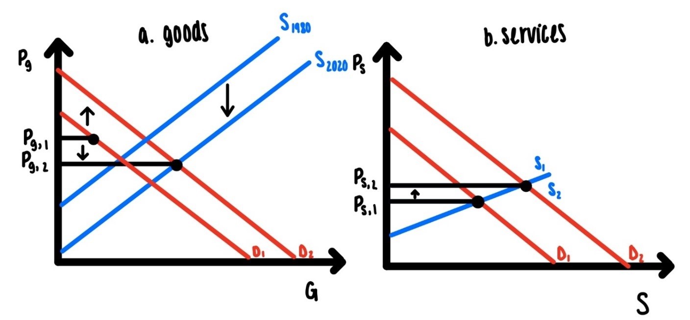
Figure 7.13: Baumols Disease II

The relative fast drop in supply in manufacturing relative to the drop in services causes manufacturing prices to drop faster than prices of services. Or, to turn this around, prices in services grow faster than in manufacturing.

The relatively fast growth in demand for services relative to manufacturing cause service prices to rise faster in services than in manufacturing.

Putting these two things together we have a veritable explosion of prices in services relative to manufacturing. This price explosion, known as Baumol’s Disease, is illustrated in Figure 7.14 below.

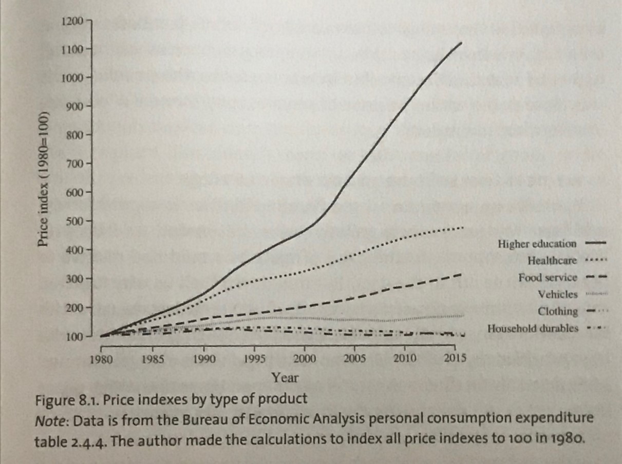
Figure 7.14: Source: Vollrath, Fully grown Why a stagnant economy is a sign of success, 2020

There are two punchlines:

As an economy gets richer, service prices relative to goods prices have to rise and it is efficient that they do.
As an economy gets richer, economic growth has to slow down and it is efficient that it does.

7.10 The Law of One Price and Arbitrage

If you look at any of the pictures of competitive markets in this chapter, you see that there is exactly one point where demand intersects supply. Since there is exactly one intersection, there is exactly one price.

This observation gave rise to what is known as

The Law of One Price

But as is the case so often, some critical assumptions that are used to derive the Law of One Price have been swept under the rug.

Sweeping things under the rug is usually not a good idea.

‘’In markets characterized by symmetric information among participants and unrestricted opportunities for resale, arbitrage assures that identical products trade at the same price.’’ - McFadden, 2023

This is how concisely one of the greats in Economics, Noble Laureate Dan McFadden⁴⁶ describes the Law of One Price. To paraphrase the statement, we can say:

If we are dealing with an object whose qualities can easily be ascertained and when there are lots and lots of trading possibilities then we would expect that object to trade at one price, at least approximately. And the availability and closeness of substitutes also matters of course.

So, if we are to analyze the Law of One Price we must consider three factors:

Information
Ability to trade
Substitutes

See, if you are selling boring Ohio State t shirts. If you sold it for $\$30$ and Jack sold it for $\$25$, then I would buy a bunch of these things from Jack and sell them for anything between $\$25$ and $\$30$ and thereby drive up the price. The price of all of these t shirts would settle somewhere between $\$25$ and $\$30$. There would be ONE price.

The Law of One Price holds.

That is the story behind the price determination in competitive markets.

But:

That is not how many markets work.

Often, we see a huge dispersion of prices. In each of the following scenarios, if you were to shop around would you see one price or a distribution of prices?

gas in Bloomington
delivery via C section in the Chicago area
shares in Ford Motor Company
one gallon of your favorite iced tea

You see the Law of One Price is not common, it is not an empirical regularity.

Whenever the law of one price does not hold, crazy things can happen. And will happen. Some are stranger than others.

First: Seek and Ye Shall Find… Maybe!

If there is a price dispersion, there will be search. Consumers will search for the lowest price. One way to think about search is that search is sequential. You can imagine you have one offer, one good with a price P at hand. The question is?

Should you buy it at that price, or should you wait, search and hope you find a better deal in the future?

That is the $\$64,000$ question.

The answer depends upon:

The current offer
Your search cost
Your expectation of prices you might find in the future
Your degree of risk aversion

It turns out that in such a case it is best for you to adopt what is called a

Reservation Price Strategy

A reservation price is a price $p^*$ such that

You accept that price if the price you have if $p < p^*$

and

You accept that price if the price you have if $p > p^*$

That means the reservation price is that price which makes you indifferent or just puts you on the fence between buying now and waiting and searching for a better deal.

That reservation price will depend on all the four factors mentioned above. If these factors change, so will the reservation price.

For example: If the search cost falls, you would be more inclined to search given your offer at hand. If you are more inclined to search, you would be choosier now. If you are choosier now, the reservation price is lower. Putting all this together:

A decrease in the search cost decreases the reservation price.

An increase in the search cost increases the reservation price.

There is a level of search intensity that is best for an individual. And it is reasonable to expect that this level of search intensity varies from person to person. It is reasonable that search costs vary from person to person. Just watch some of your friends and see how quickly they do find stuff on the internet. Or ask yourself how far it is from one drugstore to the next in Manhattan, NY or out in Manhattan, Kansas. What will your search costs be for some cough medicine, in either of these places? If people have different search costs, it is not surprising that there will be a distribution or a dispersion of prices.

The search intensity can be manipulated. McFadden mentions discounts for impulse purchases. How many times have you seen or heard of an offer that expires quickly? How many of you have seen contracts with very temping introductory offers that then are really difficult to undo?

Of course, with such strategies, all claims of efficiency of markets go out the window.

Second: Anti Price Gauging Legislation

Imagine a hurricane ripping up the Carolina coast. You don’t need a very good imagination for that. This happens pretty regularly.

There are two regions in Carolina, the oceanside and the mountains.

In normal times, that is when there is no hurricane, we would expect prices for essentials to be roughly the same. Essentials are things like bottled water, propane, etc. But right after a hurricane these prices go through the roof, probably because of a mix of supply and demand factors. Supply decreases, which increases the price. Demand increases, which also increases the price.

But this happens only in the coastal region. So now we have a large price difference between the oceanside and the mountains. Caused by the hurricane.

What do we think could happen? If you are an entrepreneur in the mountains, you might think:

Gee, I can sell water here in the mountains for $\$2$ a bottle, or I can sell it by the oceanside for $\$4$. It might be worth my while to hire a truck and ship some of that water that is sitting in my warehouse down to the oceanside.

That is called arbitrage: Buying low and selling high. Seeing an opportunity for an (almost) sure profit. Much work in the economics of finance is based on the idea of arbitrage. There, often, the working assumption is that there is no arbitrage, that there are no obvious price differentials that can be exploited, that there are no pure sure profit opportunities. For some markets this may be a good assumption. For other markets, this will definitely be a bad assumption.

If a few entrepreneurs think like that, the supply in the mountain side shifts left, the supply by the oceanside shifts right. The price in the mountains will rise, the price by the oceanside will fall.

How far?

Until the prices in both regions are roughly equated. One way to think about this is: The entrepreneurs in the mountains must be roughly indifferent between selling in the mountains and selling by the oceanside. Of course, there are transportation costs to consider.

The Law of One Price holds.

Now, enter price gouging laws. These kinds of laws often declare it illegal to raise prices substantially above levels that are considered reasonable or fair. You can see why these things will often kick in after a natural disaster like a hurricane. In such cases supply shocks often raise some prices through the roof. Such increased prices do not look fair, normal, or reasonable to many people.

Then, sometimes governments take action and invoke ‘’no price gouging laws’’. These are essentially price ceilings. So, they just do what price ceilings always do.

Keep the price low, lower than the market clearing price. But at a cost: The mandated price ceiling causes a slide down the supply curve and creates a shortage. At the mandated price ceiling, the quantity demanded exceeds the quantity supplied. There will be many households who cannot get the amenities they need, AT THAT PRICE. Frustration will set in.

You decide: Are anti price gouging laws a good idea or not?

Third: Goodbye NYC, welcome Omaha

https://www.nytimes.com/interactive/2023/05/15/upshot/migrations-college-super-cities.html

https://www.nytimes.com/2019/01/11/upshot/big-cities-low-skilled-workers-wages.html

You want to live in a nice city, close to the city center, with lots of amenities, restaurants, bars, night clubs, all that fun stuff that young professionals like to do. So, there is a choice:

Option 1: Manhattan, not the one in Kansas.

Option 2: Omaha in Nebraska.

There is a tradeoff: In Manhattan, you get all the fun that money can buy, but your abode will be very small. This is true for most big coastal cities: Seattle, Portland, San Francisco, San Diego, Boston, New York, Philadelphia.

In Omaha things are different. There may be fewer amenities, and the city may now be as ‘’cool’’ as Manhattan, but the house you can afford in Omaha is much bigger than what you could afford in Manhattan. In fact, one migrant stated that his apartment in NYC was as big as his living room in Minneapolis. That is a trade-off. That trade-off has been there all along. In fact, a study done by the Federal Reserve Bank of St. Louis documents that the average earner is about 30% better off in cities in the middle of the country than in cities on the coast.

For many years there has been a net inflow of workers with a college degree into the very expensive coastal urban areas. In the past few years that inflow has been reversed. On net, workers with a college degree are leaving these expensive coastal cities for more midwestern cities.

Questions:

Is the Law of One Price violated? Why or why not?
Can you think of three factors that can explain the recent net out-migration from high priced coastal cities? Can you state them as hypotheses? Make sure your factors are measurable.

Fourth (Actually Third ’): Goodbye Boston, welcome Lisbon/Athens

Read this article for background

You want to live in a nice city, close to the city center, with lots of amenities, restaurants, bars, night clubs, all that fun stuff that young professionals like to do. So, there is a choice:

City 1: Has a vibrant downtown area and a rich set of cultural amenities.

City 2: Has a vibrant downtown area and a rich set of cultural amenities.

In city 1 the average worker makes $\$30,000$ a year and in city 1, there are many workers that make $\$100,000$ a year.

What would you expect real estate prices to be in city 1 and in city 2?

If you are young, ambitious and if your work can be done largely online, where would you want to live?

We do indeed see a recent trend of young professionals from the US moving from City 2, Boston, to City 1, Athens or Lisbon.

Questions:

Can you think of three factors that can explain the recent net migration from cities like Boston to cities like Athens or Lisbon? Can you state them as hypotheses? Make sure your factors are measurable.
What would you expect this migration to do to Real estate prices in Lisbon? Real estate prices in Boston?
What would you expect that migration to do to the average age when young people in Portugal move out of their parents’ house into their own apartment?

Fourth: Higher Education and Airline Pricing: What a mess!

Let’s walk into a large introductory course in a public university, or even a private university for that matter. It does not matter whether it is a psychology, biology, econ, finance, or history class. Pick any two students and ask them: How much did you pay for tuition?

Or: walk up and down the aisle of any airplane on any flight between any pair of cities, A and B and pick any two passengers and ask them: How much did you pay for your ticket?

In any case: You will get two different answers, and the differences between the prices can be quite large.

Why is there such a large variation in the prices? Why is the law of one price violated so massively?

What can you say about the three conditions that are required for the law of one price to hold?

What about the symmetry of information? Who knows more, your parents or IU? Or: What does IU know that your parents might not know? Or: What do your parents know that IU might not know?

What can you say about unrestricted opportunities for resale?

What can you say about the availability of substitutes?

Fifth: If the law of one price fails, you may die

https://www.washingtonpost.com/business/2023/04/06/seniors-assisted-living-medicaid- eviction/

Think Assisted Living Facility, not Nursing Home. The Law of One Price is violated massively in assisted living facilities. Private insurance plans typically pay around $5,000 while Medicare/Medicaid pays only around $3,000. Many residents in these facilities typically use private means to pay until these are exhausted. Then Medicare/Medicaid kicks in. Folks are hoping that this arrangement will last the rest of their lives.

That is not how things work out in many cases. Often, assisted living facilities will lower the number of Medicare/Medicaid places, even if this means that long term residents who are often disabled need to be evicted. Imagine the anguish of the people about to be evicted. Imagine the frustration of people and their loved ones who have paid full price, exhausted their life savings, then switched to Medicaid funding or thought of switching to Medicaid funding, only to be told that their contracts will not be renewed, that they have to move out with a 60- day notice.

‘’Experts say moving elderly people out of familiar surroundings can induce a condition called “transfer trauma” that accelerates decline.’’

There are cases where the eviction from assisted living was followed very rapidly by death of the resident. Relatives call the forced move from assisted living a big factor in their decline.

7.11 Glossary of Terms

Competitive equilibrium: The intersection of supply and demand. This intersection determines the market price $P^*$ and the quantity $Q^*$. We will refer to $(Q^*, P^*)$ as the competitive equilibrium.

Consumer surplus: The consumer surplus for one unit purchased is the vertical distance between the price and the willingness to pay, the marginal benefit derived by the consumer from that particular unit.

Consumers’ surplus: This is the sum of all the consumer’s surpluses, summer over all goods consumed.

Excess demand: When, at a particular price, the quantity demanded exceeds the quantity supplied, we refer to the difference as excess demand.

Excess supply: When, at a particular price, the quantity supplied exceeds the quantity demanded, we refer to the difference as excess supply.

Producer’s surplus: The producer surplus for one unit sold is the vertical distance between the price and the marginal cost of producing that particular unit.

Producers’ surplus: the sum of all producer’s surpluses, summed over all goods produced.

Profit: total revenue minus total cost.

Total Revenue: the price of the product multiplied by the number of units sold.

Total cost: the cost of all the inputs required for production, including opportunity cost.

Unit taxation: a tax collected by the government on each unit of production or consumption.

7.12 Practice Questions

7.12.1 Discussion

List three positive economics questions. Discuss their importance.
List three normative economics question. Discuss their importance.
How would you determine if a particular market is competitive, using the definition from class and all your knowledge of competitive markets discussed in class? For each of the following markets discuss how competitive they are: The market for credit cards, the market for health care in Bloomington, the market for evening gowns, the market for vacations in North Carolina.
Which markets in this country come very close to being competitive? Explain your reasoning.
Which markets in this country are far from being competitive? Explain your reasoning.
In the China Syndrome example above, Example 7, what other information, if any, would be needed to estimate changes in consumers’ surplus? Explain.
In example 6 above, why is the US mostly exporting undifferentiated products and mostly importing differentiated products?

7.12.2 Multiple Choice

Imagine that there is a per unit tax of $5 on blue blouses. If markets for all blouses are competitive, then the price of red blouses will _____ and the quantity of red blouses purchases will______.

A. Rise, fall
B. Rise, rise
C. Fall, fall
D. Fall, rise
There is technological progress that makes light bulbs more durable. If light bulbs are sold in competitive markets, then the price of light bulbs will _____ and the quantity of light bulbs purchased this period will ______.

A. Rise, fall
B. Rise, rise
C. Fall, fall
D. Fall, rise
Covid 19 induced many families to move from areas with high population density to areas with low population density. Let’s refer to the first areas as cities and second as villages. The supply of real estate in cities is less elastic than the supply of real estate in villages. Then we could expect the price of real estate in cities to _____ and in villages to _______

A. Increase, increase
B. Increase, decrease
C. Decrease, increase
D. Decrease, decrease
In problem 3 above we would expect the average (over cities and villages) price of real estate to

A. Increase
B. Decrease
C. Stay constant
D. Fluctuate
In problem 3 above, consumers’ surplus in the cities is expected to

A. Increase
B. Decrease
C. Stay the same
D. Decrease only when supply is not vertical/perfectly inelastic.
In problem 3 above, suppose that supply is horizontal. The consumers’ surplus is expected to

A. Increase
B. Decrease
C. Stay the same
D. Double
Imagine that lard is an inferior good and imagine that the economy in Greaselandia goes into a major recession so that incomes drop. Then we would expect the price of lard to ____ and the quantity of lard consumed to _____

A. Increase, increase
B. Increase, decrease
C. Decrease, increase
D. Decrease, decrease
Imagine that at some number of flip-flops, the marginal benefit of flip-flops exceeds the marginal cost. Then in order to obtain an efficient output level, society should

A. Produce fewer flip-flops
B. Produce more flip-flops
C. Produce the same number of flip-flops
D. Only produce designer flip-flops
Imagine that at some point the marginal benefit of coffee is exactly the same as the marginal cost of coffee. Then a scientific study convincingly demonstrates that drinking moderate to large amounts of coffee has substantial health benefits which were previously unknown. This study is widely circulated and publicized in the media. Then we would expect the price of coffee to ______ and the quantity of coffee to ______

A. Decrease, decrease
B. Decrease, increase
C. Increase, decrease
D. Increase, increase
Which one of the following is not a consequence of rent control?

A. Lower turnover of renters
B. Longer commutes
C. Side payments for rent instead
D. Shorter commutes
When a government imposes a binding rent control then we would expect

A. Quantity demanded to exceed quantity supplied at that price
B. Quantity demanded to fall short of quantity supplied at that price
C. Quantity demanded to be equal to quantity supplied
D. The quantity traded in the market to be efficient
The efficient allocation in a market is obtained when

A. Marginal benefit is bigger than marginal cost
B. Quantity demanded is bigger than quantity supplied
C. Quantity demanded is smaller than quantity supplied
D. Quantity demanded is equal to quantity supplied
In a competitive market

A. Some firms can set the price, but household cannot
B. Some households can set the price, but firms cannot
C. Some households and some firms can set the price
D. None of the above
There is technological progress that lowers marginal cost in the production of chain saws. As a consequence, consumers’ surplus from chainsaws is expected to

A. Fall
B. Rise
C. Stay constant
D. Be twice as large as producers’ surplus
If there is free entry into a competitive market and here are currently positive economic profits to be had in that market, we would expect free entry to

A. Shift demand to the left
B. Shift demand to the right
C. Shift supply to the left
D. Shift supply to the right
We would expect fire insurance premia for homeowners in the dry states out wet over the next 20 years to

A. Increase
B. Decrease
C. Stay constant
D. Fluctuate around a decreasing trend
Atlantic state has two regions, Region 1 by the ocean and region 2 by the mountains. Region 1 is frequently hit by hurricanes. On those occasions the price of various commodities such as gasoline, bottled water, propane spikes. Laws against price gouging in Region 1 will

A. Shift demand in Region 1 to the left
B. Shift demand in Region 1 to the right
C. Shift supply in Region 1 to the left
D. Shift supply in Region 1 to the right
Which of the following does not fit?

A. Demand
B. Willingness to pay
C. Reservation price
D. Marginal cost
Which one does not fit?

A. Supply
B. Marginal cost
C. Reservation price
D. Willingness to pay
Free entry into competitive markets tends to

A. Shift supply to the right
B. Decrease price
C. Eliminate economic profit
D. All of the above

7.12.3 Answer Key

6 Supply

8 Externalities