3 Economic Growth II

In this chapter you will learn:

• The basics of human capital accumulation
• The basics of technological progress

3.1 Human capital accumulation

In the Solow model we considered in the previous sections, there was only one factor to be accumulated: physical capital. In this section we will allow for two augmentable factors: physical capital and human capital.

By human capital we simply mean all the marketable skill. In the Solow model the production function is given by \[y_t=A F(k_t)\]

Recall that when we hold labor constant, then output is basically a function of capital only and the production function exhibits diminishing returns to capital. We will now generalize the production function to

\[Y_t = A F (K_t, H_tN_t)\]

In this formulation \(N_t\) stands for labor as before. Labor could be measured by the total number of people employed or by the total number of hours worked. \(K_t\) is the total capital stock, \(Y_t\) is output of GDP and \(A\), as before is a measure of technology.

What is new here is \(H_t\), which stands for human capital. What we do here is we multiply \(H_t\) and \(N_t\) together to get

\[H_tN_t\]

We call this product “effective labor”. We can think of \(N_t\) as hours worked. If we multiply the hours worked \(N_t\) with skill or human capital \(H_t\) we can get a measure of how much can be done or accomplished in the time spent working. We will refer to \(N_t\) as “raw labor” and to \(H_tN_t\) as “effective labor”.

Effective labor varies both across countries and over time. The average Norwegian worker has more human capital and thus more effective labor then the average Nepali worker. Also, the typical American worker now has more human capital than the typical American worker had 100 years ago.

Just like physical capital, human capital can be accumulated; it can grow. It can also depreciate or become obsolete.

There are multiple ways to accumulate human capital.

• Formal schooling
• Learning on the job
• Leaning by doing

There is a large literature on each one of these components. Here we will focus on formal schooling, partially because in many countries formal schooling budgets take up large fractions of national income, GDP. In some cases, this is more than 5 or 6 % of GDP.

One way to measure formal schooling is through expenditures. How much do we spend as a fraction of GDP on formal public education? When answering this question we have to be cognizant of the fact that there is also a significant private expenditure in formal schooling.

The second way to measure formal schooling or education is simply to ask how many years of schooling do students get. Of course, in every country there will be a distribution. Often, we categorize years of schooling by the different stages of education completed, such as college completion or high school completion.

Figure 3.1. below shows that education in the US has increased tremendously. The fraction of the labor force that has completed college has increased substantially while the fraction of the labor force that has only finished elementary education or not finished high school has fallen drastically.

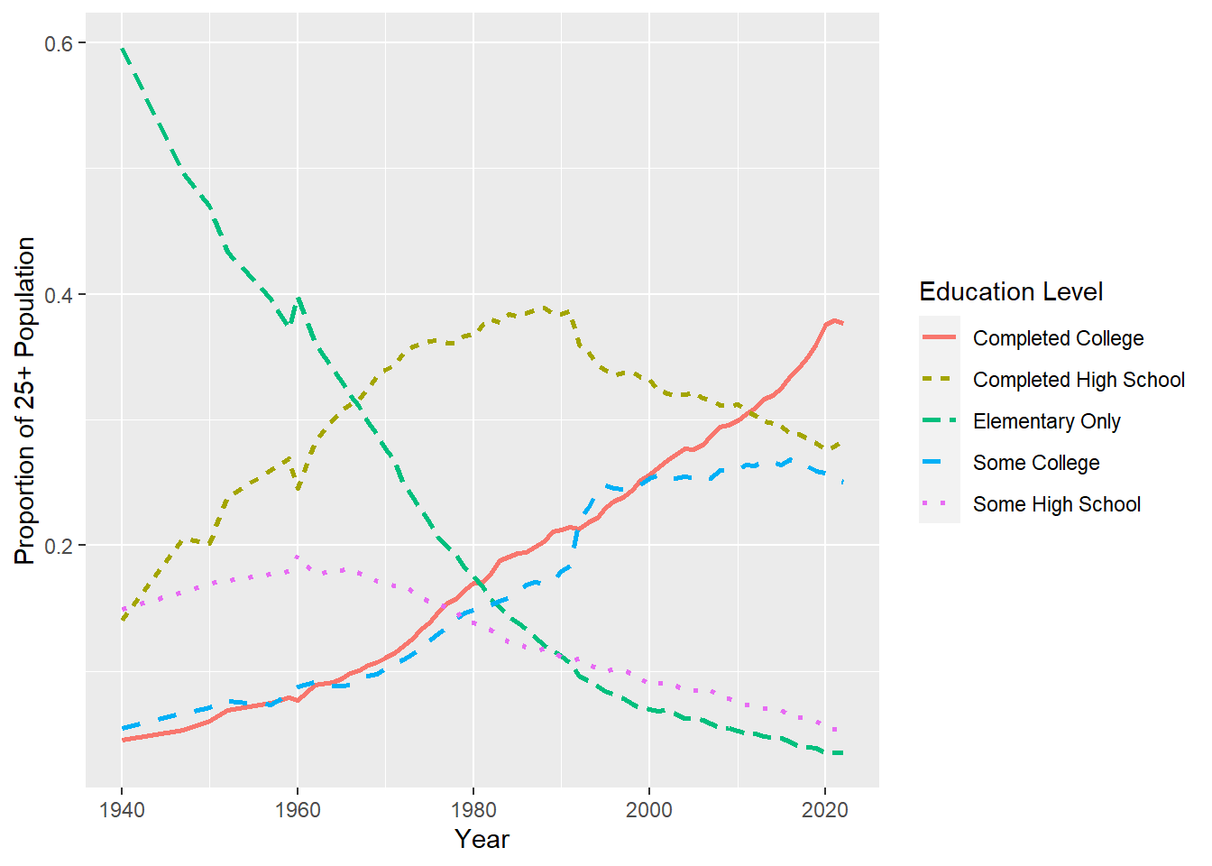
Figure 3.1: Increasing schooling time. Data Source: US Census Bureau

Most countries have seen similarly large increases in years of schooling. Measured in average or median years or schooling. Or measured in the fraction of the labor force that has completed college.

Beware of measurements!

Measurements should be useful for the purpose at hand.

Measurements should not be too costly.

Both of these are worthwhile considerations.

But, sometimes measurements are taken simply because they are cheap. Please consider the link below. There are reports from central planning in the Soviet Union by plans being fulfilled by a very small number of huge nails or, alternatively, by a huge number of tiny nails. It all depended on the specifications given by the planner to the factory.

See the cartoon below.

Figure 3.2: Source: Krokodil

Incentives work!

They work really well.

There is a similar story about shoes in the Soviet Union. People were always lining up for shoes. Always. I mean always. It turns out that the Soviet Union at the time produced hundreds of millions of shoes per year. More shoes than were produced in the US.

The problem: They were just shoes, but not shoes consumers wanted. They were just not comfortable. And forget fashionable.

So the statement above about people standing in line for shoes needs a qualification. People were standing in line not just for shoes, not just for any pair of shoes. They were standing in line for comfortable shoes, for durable shoes, for practical shoes, for shoes that fit their needs.

Why am I telling you nail and shoe stories?

In education there is the risk, that we are looking at numbers, data, measurement in a way that is very similar to the way data were looked at in the nail and shoe stories.

In education we sometimes look at numbers that are easy to collect. And sometimes these numbers are not meaningful. Or at least, it is not clear how meaningful they are.

• Years of schooling.
• The fraction of 18 years olds going to college.
• The number of hours spent studying

All these data fall into the category of questionable data. Whether data is questionable ALWAYS depends on a particular purpose: Is that data useful for my particular purpose?

So what could/would be our purpose here? We would hope that education makes people more productive. If education makes people more productive, we would see the effect of education in GDP.

Now, before we take a closer look at the connection between education and GDP, we can use some introspection to think about how useful or how accurate the above three measure can be.

Go back to high school and think of all the students who were you in graduating class. At that point they all had 12 years of schooling. Now consider the difference, if there is any, in the marketable skills among all the graduates in your class? Is that difference small? Is it large? How much do we miss in terms of productivity if for all these students, we just record 12 years of schooling?

Now think of two typical 18 year olds going to college. They are the same in all respects, expect one: Jill attends IU Kokomo; and Jackie attends Princeton. Should both Jackie and Jill be counted equally as attending college? Which one might be more productive in the labor force? How big might such differences in labor productivity be?

John and Jack both are first year students at IU. Both are studying psychology. Both John and Jack report that, outside of class, they spend 20 hours per week studying. Would/should we expect John and Jack to learn equally during those 20 hours. John concentrates on his work and Jack texts with his girlfriend, checks the stock market and pays his bursars bills while doing his homework. Should we count these two sets of 20 hours the same?

Apart from these issues, all of these are measurements of inputs, not of outputs. The outputs are what is actually learned. What are the marketable and other skills? We should care about the outputs, more than the inputs. The outputs are hard to measure, the inputs are easier to measure. So, we will measure the inputs.

Hanushek and Kimko in their paper from 2000: Schooling, Labor-Force Quality, and the Growth of Nations make a big effort to get this right. For a bunch of countries, they look at the correlation between years of schooling and economic growth. They do find a positive correlation, exactly what one might expect. But correlation allows for causation in both directions: More years of schooling could imply higher growth. Higher economic growth induces people to get more schooling. So inferring causality from more years of schooling to economic growth is dicey.

There is more. We actually have data on math and science scores of students at the high school level that are comparable across countries. This is a measure of an output, things that students actually learned and know. As an aside, the US performance in these international tests is very mediocre.

If we introduce this measure of student scores in our statistical analysis of schooling and economic growth, the correlation between years of schooling and economic growth goes to zero and the correlation between learning scores and economic growth is positive. And it is large. Very large.

A one standard deviation increase in these test scores is associated with a 1.4% increase in the growth rate. This is huge. Recall that for the longest time the growth rate of real per capita income in the US has been 1.8% annually. So, if, somehow magically, or perhaps less magically by prudent choice of education policy, the test scores of US students could be increased by one standard deviation, then the long run growth rate of GDP would be increased by 1.4% from 1.8% to 3.2%. That is big. Very big.

Imagine that we start with an income of $60,000. In one case we have a growth rate of 1.8% and in the other case we have a growth rate of 3.2%. Then we have income after 10 years

\[\$60,000 (1.018)^{10} = \$71,718 \]

\[\$60,000 (1.032)^{10} = \$82,214\]

A ten thousand dollar difference is large, by any stretch of the imagination. We could have made this appear even bigger by calculating differences twenty of thirty years out.

There are two more stunning observations that come out of the above paper.

1. Economic growth in that sample of countries is uncorrelated with public expenditures on education.
2. The test scores in that sample of countries are uncorrelated with public expenditures on education.

Putting these two things together means that the amount of resources does not matter that much. What matters more is what you do with them.

3.2 More Human Capital

It is well to consider the correlation between PISA scores and economic growth as done by Hanushek and Kimko, but there is certainly room to do more. Perhaps one can really construct a measure of that H variable that shows up in our production functions, or at least a proxy.

This is done by Egert et al. (2022)³³.

First: The PISA scores measure what 15 years old know. Much of that knowledge might disappear before these youths reach their productive years in the labor force. There is a measure of adult knowledge called the Programme for the International Assessment of Adult Competencies, PIAAC. This measures adult literacy, numeracy and problem-solving skills. As a drawback this is only available for relatively few countries. Egert et al. show that PISA scores and PIAAC scores are highly correlated. So, they can use the PISA scores in their attempt to construct a measure of human capital.

Second: Then Egert el al. constructs their measure of human capital for about 80 countries by combining PISA scores and median years of schooling. And there is one more issue. If we look at the US or any other labor force now, we are looking at 20-year-old workers, 65-year-old workers and workers of all ages in between. The 20-year olds were 15 just 5 years ago. The 65 years olds were 15 years of age 50 years ago in 1972. So, we have to average all these PISA scores over all these ages or cohorts. When we do this, the US is sort of in the middle of the pack just above Austria, Hungary, Spain and Italy but below these countries:

France, Slovakia, Belgium, Sweden, Poland, Czech Republic, etc.

The highest countries by this measure are: South Korea, Finland, Japan.

Third: Their constructed measure of human capital is highly correlated with Total Factor Productivity. That is the A in our production functions. This is illustrated in Figure 3.3 below.

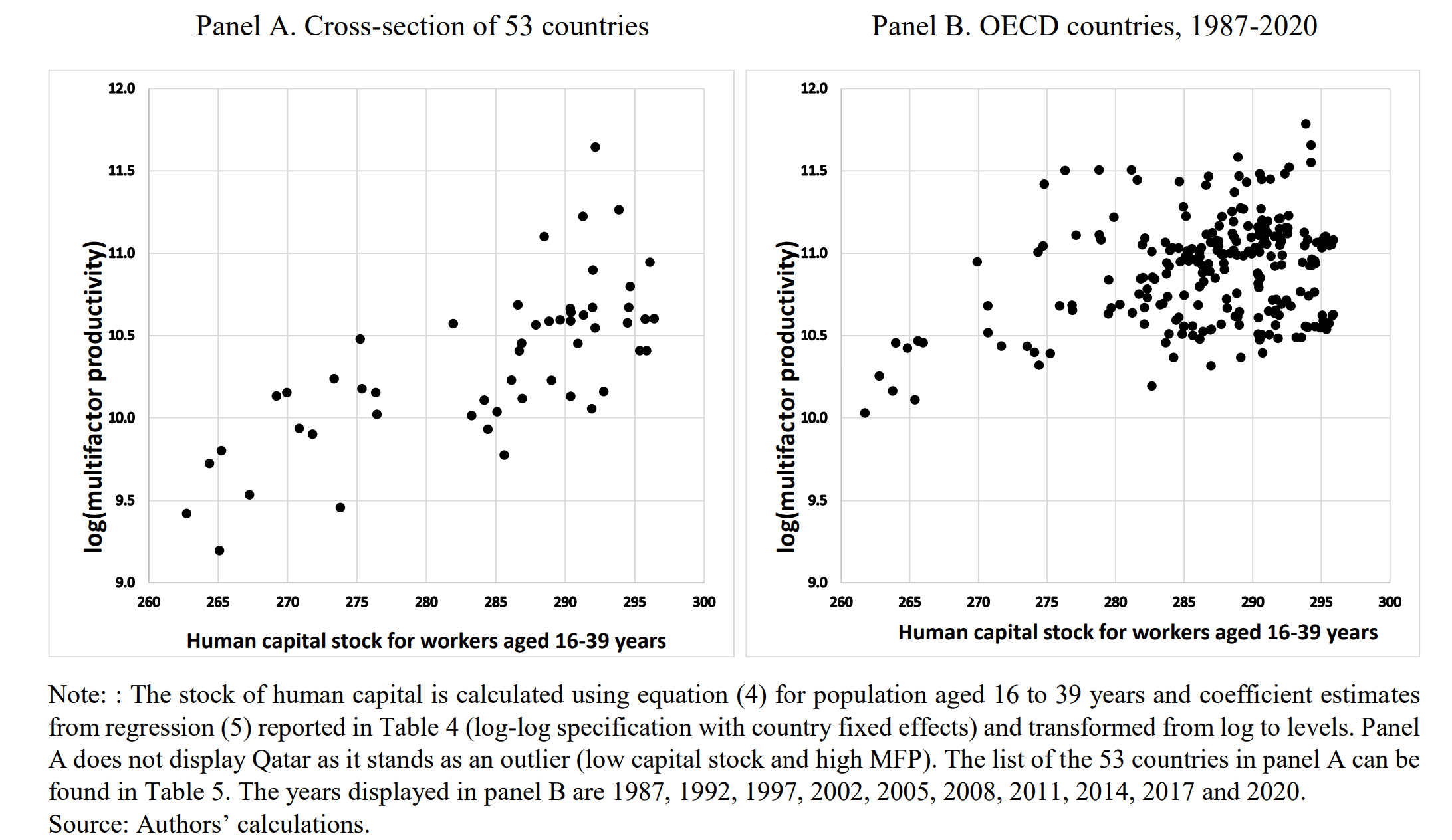
Figure 3.3: Taken directly from Egert et al (2022) Figure 5

Fourth: Which aspect of human capital, the PISA score or median years of schooling is more important for increases in productivity? It turns out the effect of increasing PISA scores is about twice as big as the effect of increasing median years of schooling.

Fifth: Early childhood intervention

There is a large literature by now on the effects of early childhood intervention. Heckman et al. (2010) is just one example. So, what is early childhood intervention? Substantial education programs for children at risk and their moms. There is a lot of evidence that the rate of return, the benefit-cost ratio, the bang for the buck is increasing the younger are the students. It is truly very large for the youngest students, three and four year olds. The US is near the bottom of this distribution. See Figure 3.4.

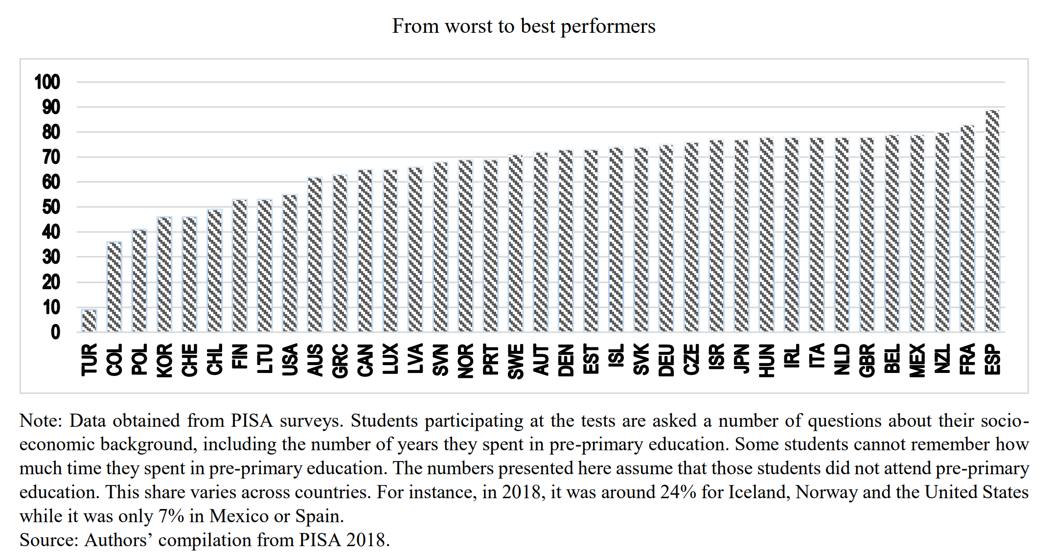
Figure 3.4: Taken directly from Egert et al (2022) Figure 7

Egert et al. show that improving early childhood education can have very large positive effects on future productivity. Perhaps this is not that surprising. Of course, we will have to wait a bit for these effects to kick in. After all, it will take a while for these kids to grow up and join the labor force. But good things are worth waiting for.

These effects are especially large at the bottom of the early childhood schooling distribution, where the US seems to dwell. Which of course raises the question: Why is a rich country like the US not doing more to improve early childhood intervention?

3.3 Technological progress

We write the production function as

\[Y_t = A_t F( K_t, H_tN_t)\]

where the subscript t stands for the time period and the symbols Y, A, K, H, N stand for, in order output/GDP, productivity, physical capital, human capital and labor time/ hours worked. So far, we have addressed the growth of physical and of human capital. That leaves the question:

• How does productivity grow?
• What factors influence the growth of technology?
• What factors influence technological progress?

We will use the simplest possible model to give an answer to this question.

Note that I did NOT say that I will answer this question. I said to “provide an answer”. There are many ways to provide SOME answers.

One simple way to provide an answer is simply to assume that the new ideas that generate technological progress are created by hiring workers to create new ideas. These workers are called, surprise, surprise, scientists. We let \(S_t\) denote the number of scientists hired, then we posit that technological growth is described by

\[ \frac{A_{t+1} - A_t}{A_t} = B S_t \]

The left-hand side is the percentage growth of productivity. The right-hand side is just the resources allocated to research. This could include the number of scientists employed, perhaps weighted by their human capital, but also the labs, the buildings for the labs, the lab equipment, and supplies and energy to run the lab experiments. The relationship is very simple: The more resources allocated to science, the higher is economic growth. B is a measure of productivity in research. More precisely, as specified, this relationship is linear. A doubling of resources leads, in this specification, to a doubling of the growth rates. This is an assumption; the world does not have to look like this.

We must keep in mind that there is a feasibility or adding up constraint. There is a total number of workers in an economy. They can be either production workers or scientists/researchers who produce ideas. If we let N be the fraction of production workers and S the fraction of scientists, then we must have

\[ N + S = 1 \]

where 1 is the total number of workers. That number cannot be exceeded.

We can now take a look at technological progress in a few sectors. Perhaps the most celebrated example of technological progress is Moore’s Law. Moore’s law was promulgated in the early 1970s by Gordon Moore, one of the co-founders of Intel, and meant as a forecast that the number of transistors on an integrated circuit, perhaps we can think of this as computing power, would double ever 2 years. This “law” stood the test of time. Over the last 40 years this relationship has held up very well. Note the scale on the vertical axis in Figure 3.5. In 40 years going from 2,300 in 1971 to 2,600,000, 000. That is nothing short of spectacular.

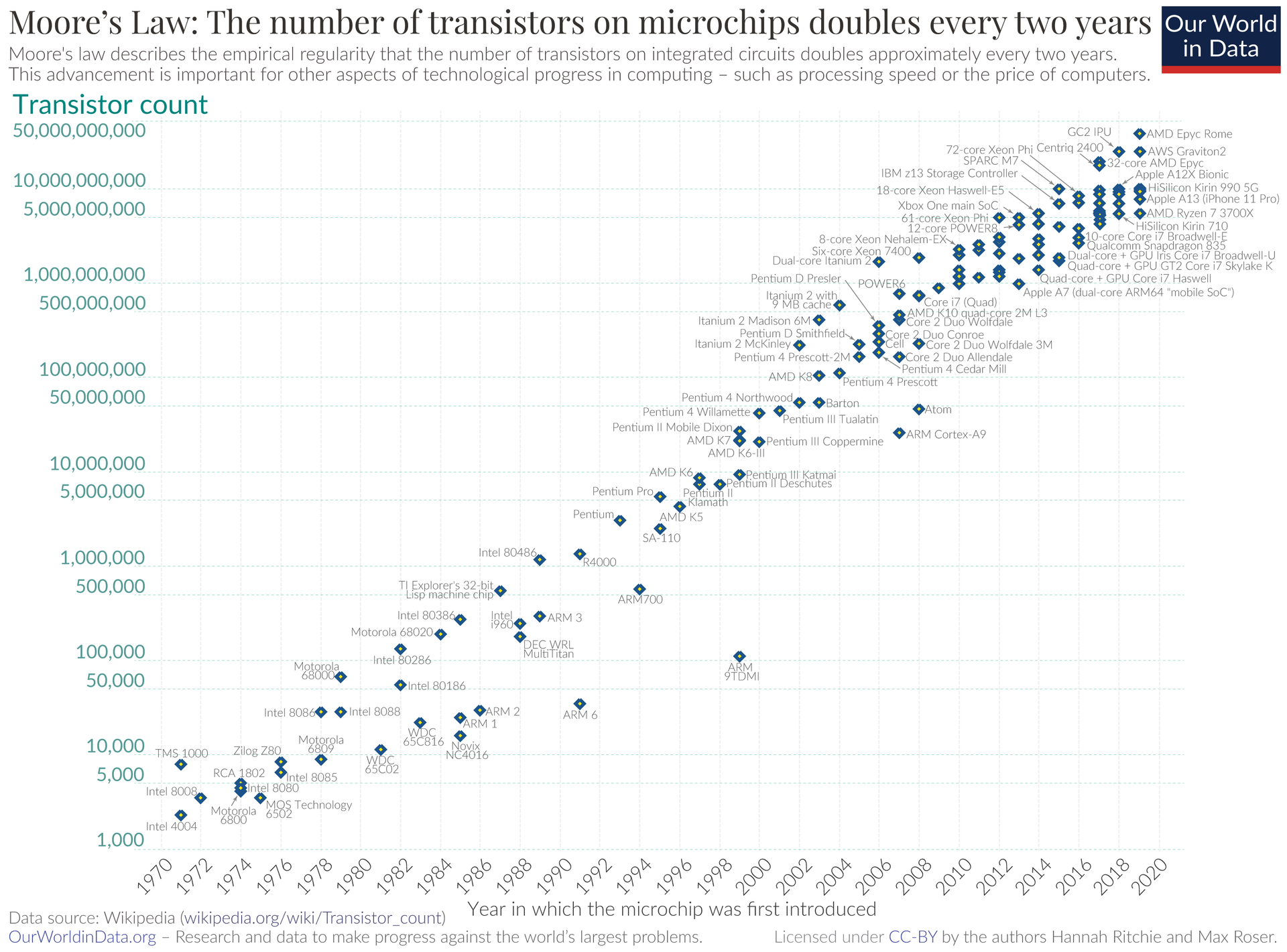
Figure 3.5: Moores Law

Considering that graph above, one could be very optimistic. There does not seem to be any break in that trend. The best fit in these data points seems to be a straight line with constant slope. Since the scale on the vertical axis is logarithmic, this looks like exponential growth at a constant rate. If there were no extra information one could become quite sanguine and expect constant exponential technological progress to continue.

Alas, there are other things to consider. What did it take to maintain the incredible growth of computing power summarized by Moore’s law?

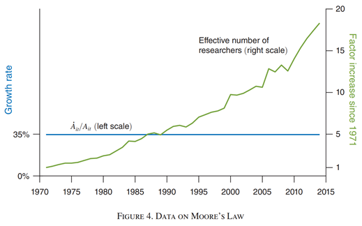
Figure 3.6: Moore’s law requires huge increases in the number of researchers. Source: Charles I. Jones Annu. Rev. Econ. 2022. 14:125–52.

Figure 3.6 shows that over time the number of workers/scientists required to maintain Moore’s law want up by a factor of 20 over that period.

A factor of 20!

We can conclude from these two numbers that back in the 1970s, it was easier to double every two years. Now it is harder to double. It takes more resources to double.

That is diminishing returns.

There is no hint in the data, the two series in Figures 3.6, that future doubling will require fewer inputs.

We picked the low hanging fruit first. Now we got to climb higher.

Figure 3.7 shows something similar for agriculture: Yields per acre have been growing, but at declining rates but the number of researchers has been rising tremendously. Wheat, corn, soybeans, cotton; its all the same story.

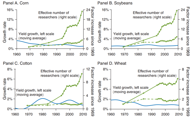
Figure 3.7: For agriculture it seems the same holds true. Increases in productivity come at an ever increasing resource requirement. Source: Charles I. Jones Annu. Rev. Econ. 2022. 14:125–52.

Low hanging fruit was picked long time ago.

Figure 3.8 panel b shows the same story for mortality or survival from breast cancer. Mortality rates are way down, and they are declining, albeit at declining rates. Research effort measured by scientific publications and clinical trials are way up.

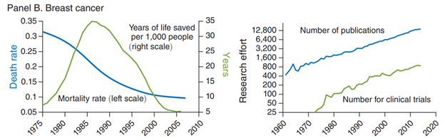
Figure 3.8: For health again it seems the same holds true. Increasing productivity comes at the cost of ever increasing resource requirements. Source: Charles I. Jones Annu. Rev. Econ. 2022. 14:125–52.

Same old song: Low hanging fruit was picked years ago.

Figure 3.9 shows how drastic these diminishing returns are. Peak productivity was reached around 1990 when one clinical trial was responsible for about 16 life years saved per 100,000. Now we are down to 1.

A drop from 16 to 1.

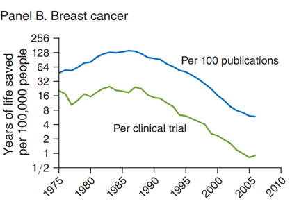
Figure 3.9: Diminishing returns to breast cancer after 1985. Source: Charles I. Jones Annu. Rev. Econ. 2022. 14:125–52.

Most low hanging fruit seems to be gone. If we want to get any fruit, we got to climb REEEEAAAAAALLLLLLY high.

Since there seem to be many industries where technological progress is only achieved with the help of ever-increasing numbers of scientists it is a fair question to ask whether this is true also in the aggregate, i.e., for the total economy.

The answer to this question is a resounding YES. Figure 3.10 shows aggregate technological progress for the US economy over a 70-year period starting with the 1930s. The pattern is clear: There is no increase at all in the rate at which technology has progressed. If anything, there is a declining trend.

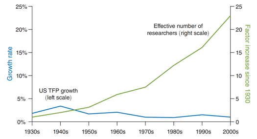
Figure 3.10: Constant or declining productivity growth has required ever more researchers. Source: Charles I. Jones Annu. Rev. Econ. 2022. 14:125–52.

Figure 3.10 shows that this rise in productivity (at a declining rate) has been accomplished by an increase in researchers in the order of a factor of 20! This is huge.

Just like at the level of individual industries or activities, there is no evidence that these trends will be reversed. We can, with some degree of confidence, predict that future economic growth will be lower than past economic growth.

Those politicians running for election, who promise to make the economy grow at 3 or 4% annually, have to work really hard to fulfill their promises since they are working against strong headwinds that are basically beyond their control.

(All the above figures are from the first paper listed below.)

The second paper below addresses the questions:

• What factors are contributors to the growth of real per capita GDP or output for short? And how important are they?
• What factors are contributors to technological progress or the growth in productivity? And how important are they?

Given the production function specified above, we can decompose the growth in output into the following components:

1. Changes in the ratio of capital to output
2. Changes in educational attainment/ growth in human capital
3. Changes in the employment to population ratio
4. Changes in the fraction of workers in production rather than research.

How big is each of these factors? Jones (2021) provides the estimates. In the US starting in the 1950s, an increase in fraction of people employed is responsible for growth of 0.2%, the increase in human capital per person is responsible for growth of 0.5%, and technological progress contributes 1.3% for a total of 2% annual real per capita growth. Punchline: productivity growth or technological progress is responsible for the biggest part of growth.

What is the potential for future economic growth?

It seems difficult to imagine that educational attainment can still increase substantially. In the US, median years of schooling increased relatively rapidly until about 1980, but then the curve flattened out and that growth diminished. It is unlike that that growth will increase in the near term.

We are already hiring more and more researchers to generate more ideas with diminishing returns. Hiring more and more researchers comes at a cost of fewer workers in production with a corresponding current output decline. It seems hard to think of factors that can turn the declining research productivity around.

How about population growth? As the population grows, there are potentially more researchers as well. But population growth rates are falling worldwide?

Perhaps we can do a better job identifying and fostering future Einsteins and Curies? According to some estimates only 12% of inventors are women, while roughly half of the population is women. Policies that increase that number might increase growth by 0.3%.

https://web.stanford.edu/~chadj/dignity.pdf

https://web.stanford.edu/~chadj/annualreview.pdf

3.4 Nails

Sometimes we see something very extra ordinary in something totally ordinary. But I think that is true in life in general. Sometimes we see it. Sometimes we don’t.

Nails are very ordinary. Our lives are made much better by nails. All of our kitchen cabinets, let alone our houses, are all held together by nails.

So, what is so remarkable about nails?

It is the prices!

Sichel (2022) has put together a long data series on nail prices. See Figure 3.11 below.

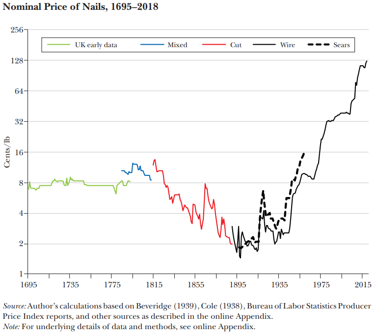
Figure 3.11: Taken directly from The Price of Nails Since 1695: A Window into Economic Change by Daniel Sichel (Journal of Economic Perspectives 2022), Figure 2

But you will say: what is unusual about this? The price is kind a constant, then drops then rises. We all know that prices always fluctuate.

But let us not been that dismissive that quickly. The prices in that figure are nominal prices. We should probably correct for inflation and for changes in nail quality. Nail quality would be something like “holding power”.

If we do this, we get a series of nail prices as in Figure 3.12.

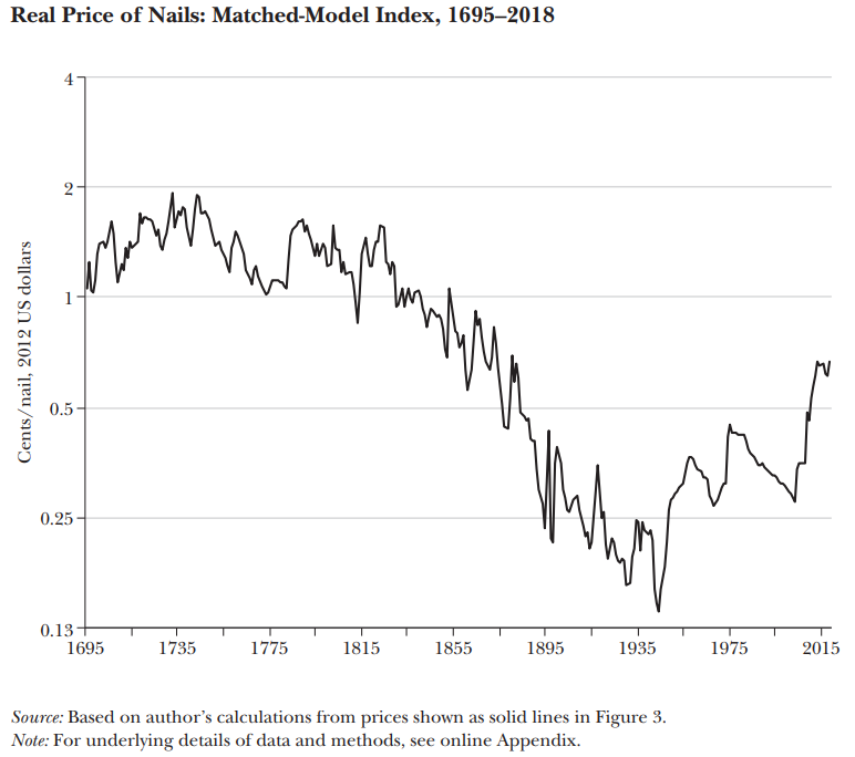
Figure 3.12: Taken directly from The Price of Nails Since 1695: A Window into Economic Change by Daniel Sichel (Journal of Economic Perspectives 2022), Figure 4

The drop in prices between 1695 and 1935 is spectacular: The price has dropped from almost 2 cents a nail to about 0.15 cents a nail. That is drop by a factor of 10!

Why would the price drop so much?

There typical reasons are:

• The availability and prices of inputs in the production of nails.
• The quality of such inputs.
• Total factor productivity.

So, what is the lions’ share of the reasons for this large drop in the price of nails? It is total factor productivity. That factor is so large that it totally overwhelms the other factors. The periods where total factor productivity really had its biggest kick are the periods where rapid technological change happened such as the switch from steam to electricity.

3.5 Light

https://www.nber.org/system/files/chapters/c6064/c6064.pdf

What a miracle. You wake up in the morning in January and you flip a switch, and voila, you can see, dimly because you are not quite awake, but you can see; you can see because there is light.

It has not always been like that. Our early ancestors struggled mightily to get some light by making a fire so they could see.

Over thousands of years things have changed and improved. We went from collecting firewood and rubbing stones together to flipping a switch.

These technological advances involved changes from the open fires to lamps, to candles, to gas and petroleum, to electric lighting, and from carbon to tungsten filaments.

These historical developments are listed in Table 3.13 below

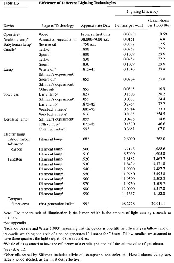
Figure 3.13: Taken directly from Do Real-Output and Real-Wage Measures Capture Reality? The History of Lighting Suggests Not by William D. Nordhaus (NBER 1996), Table 1.3

Before we follow the historical development of these technological improvements, we need to fix few terms.

• Light is radiation that stimulates the retina.
• Light flux or flow is the rate of emission from a source.
• The unit of light flux is a lumen.
• The unit of illuminance, the amount of light per unit area, is the lux.

All of this is physics so far. We need to get to the economics…

We are interested in the price of a lumen hour. The price is an imperfect measure.

There are many factors which influence the price. There are input prices that can increase or decrease over time. There is technological change. Getting the price changes right is crucial. The price of light of course depends on the price of inputs. Between 1883 and 1983, the price of gas and kerosene rose by a factor of 10 and the price of electricity fell by a factor of 3!

Adjusting for quality is another major issue. Just imagine sitting by the light of two candles in the UK in the 1700s and doing your algebra homework. Or imagine your parents paying a slew of medical bills over an open fire pit.

If you do all these things carefully, you can constrict price of light data for the last 200 years. This is exactly what Nordhaus did in 1996. His results are in Figure 3.14 below.

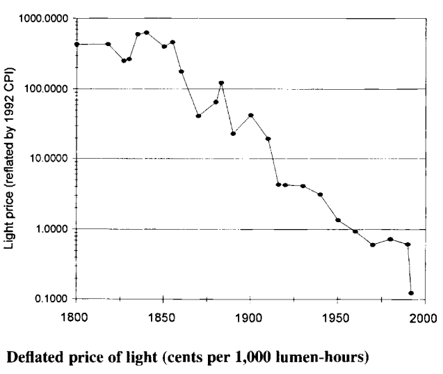
Figure 3.14: Taken directly from Do Real-Output and Real-Wage Measures Capture Reality? The History of Lighting Suggests Not by William D. Nordhaus (NBER 1996), Figure 1.3

That is an impressive drop. From almost 1000 to about 0.1.

Three cheers for technological progress!

3.6 Additive Growth

So far the basic underlying assumption in everything we have done is that

growth is exponential.

A recent paper by Philippon (2022) casts grave doubt on this assumption. We briefly lay out his main arguments here.

Imagine that technological progress is the main driver of economic growth. We can and we have modelled technological progress as

\[\begin{equation} A_{t+1}=A_t(1+g) \tag{3.1} \end{equation}\]

Here, of course, \(A_t\) is the level of technology and \(g\) is a positive number. This equation just says that the growth rate of technology takes the current level of technology and multiplies it by some number. This is all well and good and it sounds very reasonable. And a bunch of economic research going back all the way to Solow (1956) has made and used this assumption.

But:

It would just have been as reasonable to assume and write

\[\begin{equation} A_{t+1}=A_t + b \tag{3.2} \end{equation}\]

Equation (3.1) is multiplicative; Equation (3.2) is addititve.

There is no “a priori” (you may want to look this up) reason to believe that one of those two equations is a better assumption for research on economic growth than the other.

So how do we distinguish one model, one assumption, one theory from another?

We use data. At least we try to use data.

This is the approach social scientists take in many areas of live: using data to distinguish theories.

Here is another example:

Suicide incidence in the US is very high.

Theory 1: It is a mental health problem.

Theory 2: It is a gun availability problem.

Question: What is the best data you can use to distinguish between these two theories?

Back to growth.

How does Philippon (2022) use data to distinguish Equations (3.1) and (3.2)?

First, he takes data on total factor productivity (TFP) the \(\{A_t\}\) series in the models for the US from 1947 to 2019. He hires two statisticians, George (for geometric growth), and Daniela (for addititive growth). He gives them the sample from 1947 to 1983 and asks them to forecast the data up until 2019.

Their answers are below in Figure 3.15

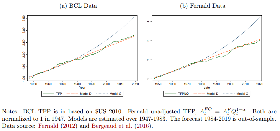
Figure 3.15: Taken directly from Additive Growth by Thomas Philippon (NBER 2022), Figure 1

The data (reality) is the solid line. George’s forecast is exponential (Equation (3.1)) and is way off.

It appears that Daniela’s forecast, using Equation (3.2) is much better.

But growth here in it’s additive form is not constant over very long horizons. Consider Figure 3.16 below

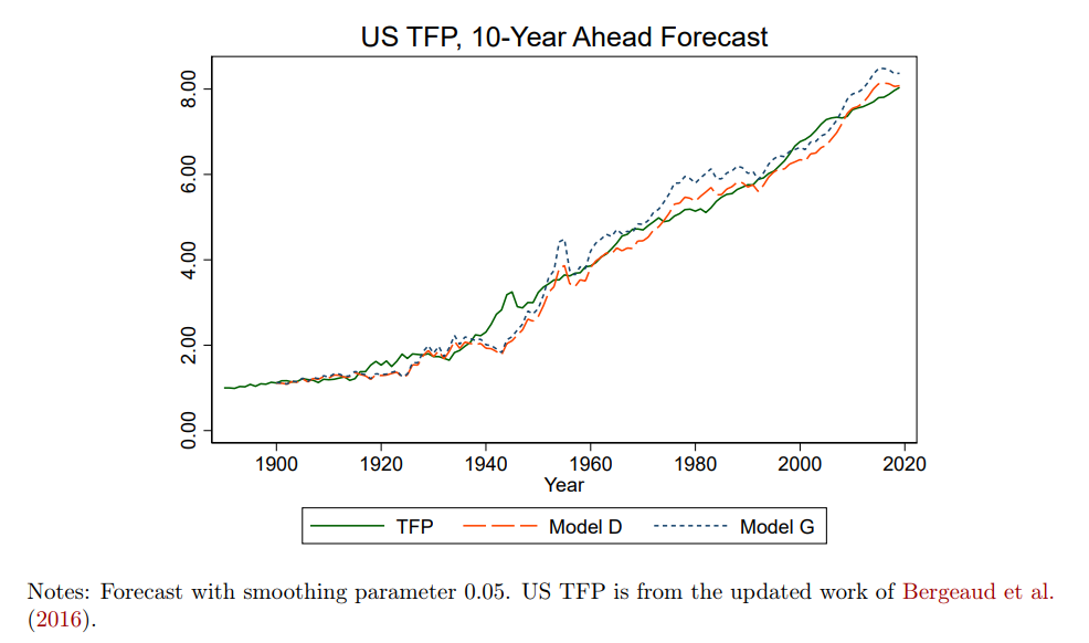
Figure 3.16: Taken directly from Additive Growth by Thomas Philippon (NBER 2022), Figure 4

There is a definite break in the data in the 1930s. Field (2003) argues that

“the years 1929-1941 were, in the aggregate, the most technologically progressive of any comparative period in US economic history.”

Perhaps this timing is a bit of a puzzle since what we consider to be many of the great drivers of technological progress, electric light, electric power, and the internal combustion engine were all discovered much, much earlier.

But the 1930s were a period of great “follow-on inventions, such as the perfection of the piston power-powered aircraft and television, and the increasing quality of machinery made possible by the large increases in available horsepowers and kilowatt-hours of electricity.” (Philippon 2022, p26) These follow-on inventions powered technological progress since.

The punchline: The constant average additive growth after the 1930s is over three times as high as before that period.

All the way to the year 2020.

Why does any of this matter?

There has been much talk, discussion, punditing, and even economic research on

the productivity slowdown.

And along with this discussion of the productivity slowdown, come all kinds of well and ill informed policy proposals:

Change education

Lower Taxes

Ease the Regulatory Burden

Etc.

Etc.

Etc.

IF growth is not exponential, IF growth is indeed linear, then Phillipon says

There is no productivity slowdown

and all the above policy discussions are moot.

3.7 Glossary of Terms

Human Capital: the stock of marketable skills of the labor force in a country.

Technological Progress: increase in total factor productivity.

3.8 Practice Questions

3.8.1 Discussion

3.8.2 Multiple Choice

1. The best measure of human capital in an economy is

   A. The fraction of workers with a college degree
   B. The fraction of workers with a high school degree
   C. Test scores of students in math and science
   D. The high school drop out rate

2. The best measure of human capital in the labor force in United States in the year 2015 is

   A. Test scores in math and science of workers who entered the labor force in 2010
   B. Test scores in math and science of workers who entered the labor force in 1970
   C. Test scores in math and science of workers who entered the labor force in 1950
   D. Test scores in math and science of workers who entered the labor force between 1970 and 2010

3. In the data set used by Hanushek and Kimko (2000) which pairs of data across countries are correlated

   A. Education expenditure per student and test scores
   B. Education expenditure per student and growth rates of GDP
   C. Growth rates of GDP and test scores
   D. Growth rates of GDP and median years of schooling, after correcting for the math and science scores

4. If the process of economic growth is linear as claimed by Philippon, then the percentage growth rates over time will be

   A. Increasing
   B. Decreasing
   C. Constant
   D. Oscillating

5. Imagine that in the years 1980, 1990, 2000, 2010 and 2020 the 5 year mortality rates from colon cancer are 45%, 40%, 35%, 30% and 25%, respectively. The number of researchers employed in these years is 100, 110, 121, 133, 147. If we consider the percentage reductions in mortality rate the research output, then this example displays

   A. Constant returns to research
   B. Decreasing returns to research
   C. Increasing returns to research
   D. Initially increasing and then decreasing returns to research

6. Imagine that human capital and physical capital are equally important in the production of output. The growth rate of human capital is 4% per year and the growth rate of physical capital is 2% per year. Then the annual growth rate of output will be in percent

   A. 2
   B. 3
   C. 4
   D. 5

7. Imagine that physical and human capital are constant over time and that there are diminishing returns to research. Then we should expect

   A. GDP growth rates to decrease over time
   B. GDP growth rates to stay constant over time
   C. GDP growth rates to increase over time
   D. GDP growth rats to fluctuate over time

8. Imagine that the stock of physical capital grows at 2% annually, that the stock of human capital is constant. If there are diminishing returns to research, then we would expect that

   A. The growth rate of GDP converges to 2% over time
   B. The growth rate of GDP is constant at 2%
   C. The growth rate of GDP converges to 0% over time
   D. The growth rate of GDP converges to 3% over time

9. Which one does not belong

   A. A new and improved surgical instrument
   B. A more fuel efficient car
   C. Better graphics for video games
   D. More varieties of soft drinks

10. Which one does not belong

    A. Electricity
    B. A fork lift
    C. A warehouse
    D. An algorithm