8 Externalities
In this chapter we will learn:
- The definition of an externality
- The distinction between positive and negative externalities
- The (in)efficiency properties of competitive markets in the presence of externalities
- How and to what extent government policies can be used to make competitive equlibria with externalities more efficient
8.1 Introductory Videos
8.2 Negative Externalities
About 10,000 people die each year in the US in alcohol related traffic accidents. Among those victims are about 200 children below age 14 47. The annual cost of alcohol related crashes amounts to about $45 Billion. That amounts to $140 per person in this country. And these numbers do not include any component due to the loss of life, what economists call the “statistical value of a life”. Nor do these numbers include the emotional suffering and grief and potential follow up costs such as grief counseling or therapy.
Where are these losses, where are these costs in our analysis? If you look at Figure 4.3 in Chapter 4, you would be hard pressed to find these costs, to find this suffering.
In Figure 4.3, the demand curve reflects the marginal benefit of the good, the supply curve reflects the marginal cost.
We must make an important clarification and distinction.
The marginal benefit in that figure is private; it is the private marginal benefit. If I eat a slice of pizza, the marginal benefit from that slice is mine. It is private. It does not accrue to anyone else. We will call it
Marginal Private Benefit, MPB.
Similarly for supply. Supply is marginal cost, private marginal cost. The marginal cost of beer is the cost of the hops, the yeast, the water, the bottle or can, the barley, etc. These are the costs of the brewery. They are no one else’s costs. They are private to the brewery. We call it
Marginal private Cost, MPC.
In the competitive equilibrium in the previous chapter, marginal social benefit, MSB, is balanced or equated with the marginal social cost, MSC. That is exactly the efficiency condition in competitive markets; when MPC = MPB, then the competitive equilibrium is said to be efficient.
But the 200 children and other innocent victims of alcohol induced traffic fatalities are not in the picture yet. We will remedy this situation now.
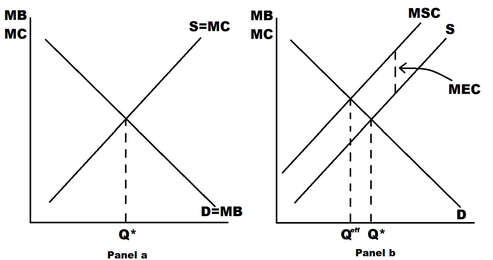
Figure 8.1: Adding social costs.
In Figure 8.1’s Panel a we reproduce Figure 4.3 from chapter 4. In Figure 8.1’s Panel b we finally confront the kinds of costs mentioned at the beginning of the chapter.
We call these costs
External costs.
These costs of being killed by a drunk driver are external costs, they are external to the decisions to make alcohol and the decisions to buy and consume alcohol. That child that gets run over and killed by a drunk driver while on her way to the children’s’ museum with her mom has nothing to do with the demand and supply decisions for beer.
What is going on here is: There are some people who engage in an action or transaction and that action/transaction has an effect on innocent bystanders. This effect is called an
externality
external effect.
And, since that externality imposes a cost on others it is called a
negative externality.
In Panel b, there are the usual demand curve, MPB, and the usual supply curve, MPC. In additions to these curves is the curve indicating
Marginal social cost.
The vertical arrow between marginal private cost and marginal social cost is the
Marginal external cost.
Marginal social cost, \(MSC\), is just the sum of marginal private cost, \(MPC\), and marginal external cost, \(MEC\).
\[MSC = MPC + MEC\]
So, what is going on in Figure 8.1’s Panel b? The intersection of MPB and MPC is still the intersection of demand and supply. It is still the equilibrium. That is exactly as before.
However:
The efficiency property of the equilibrium has changed.
When we consider efficiency, we have to look at all costs, the private and the external costs. If you are running a company in the pursuit of maximum profit, you would have to consider all costs. It would not be permissible to take one random component of costs and ignore it. It would not be legitimate to ignore the cost of unskilled labor or the cost of maintenance or the cost of replacing outmoded equipment. You would look at all cost.
Same here.
In the pursuit of efficiency, we consider all costs, the private and the external costs.
Efficiency requires that marginal social cost is equated with marginal benefit side. Note here there are no differences between private and social benefits. There are no external benefits in this particular example.
So, equating marginal benefit to marginal social cost yields the efficient allocation. We call if \(Q^{eff}\), where eff stands of course for efficiency.
The equilibrium is, as before, \(Q^*\).
We see
\[Q^{eff} < Q*\]
In words, the equilibrium allocation is bigger than the efficient allocation.
In other words: We have over production.
The market gives us too much stuff.
The equilibrium is not efficient.
Adam Smith’s Invisible Hand has failed.
When the markets fail to deliver efficient outcomes is we speak of
“market failure.”
Why does this market failure happen?
Why? Why? Why?
The reason is actually quite simple.
We have over production, since none of the firms take into consideration only the private cost, but not the external costs.
This recognition directly leads to a policy recommendation to solve this inefficiency problem:
Since the market participants do not take the external costs into consideration, the costs they consider are too low. So, in order to fix this situation, we need to raise costs. We know how to do that. We can raise a particular kind of tax. This tax is called a
Pigouvian tax
named after Arthur Pigou48, who is widely credited with introducing this particular policy.
8.2.1 Pigouvian Tax
How does the Pigouvian tax work?
Imagine a scenario where the marginal external cost is \(\$10\). The a per unit tax on firms would increase their marginal cost by exactly \(\$10\). Then the firms private marginal cost with the taxes would be exactly equal to the marginal social cost. Then the equilibrium would be exactly at \(Q^{eff}\). The equilibrium with Pigouvian taxes is efficient.
We illustrate how such Pigouvian taxes work in Figure 8.2 below.
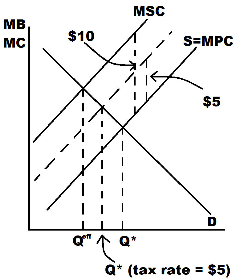
Figure 8.2: Illustration of Pigouvian tax
The supply curve is the marginal cost curve. If we levy a per unit tax of \(\$5\) on the firm its supply curve with shift to the left. Then the intersection with demand, which is marginal benefit, will shift to the left as well. To the left and up.
If we were to gradually increase the tax, we would be moving to the left and up along the demand curve. You can see where this is heading.
If the external effect on the margin is \(\$10\) and if the Pigouvian tax is \(\$10\), then the competitive equilibrium with the tax is efficient.
The problem is solved.
In theory, they say. And here that is absolutely true. In theory.
There are all kinds of practical problems.
How exactly do we determine the marginal social cost? Consider the external costs imposed by the coal fired power plants in the upper Midwest on people and on the environment further to the east. How can we asses that impact on human health, the quality of life and longevity? How can we assess the damage to rivers, to forests? Etc? And then attach a dollar value to that?
This seems hard and this is just one issue.
Imagine that you are asked to assess the external costs of global climate change. A recent study by Deloitte puts the cost of global warming at \(\$178\) trillion over 50 years. Measuring the total global cost of global warming over a 50-year period and assigning one cost number to that, sure is non-sensical. The well-paid consultants ought to know that. If not, they may go back to their universities are asking for their tuition money back. Matthew Kahn 49, carefully explains why such a practice is just wrong. See below.
Just because we cannot and should not attach one single number to these external costs, does not mean that we should not levy a Pigouvian tax, in the case of global warming, a carbon tax. We can start with a low tax rate, that might correspond to some lower estimates of the external costs, and then gradually increase the tax rate over time.
The external costs are not necessarily constant as in Figure 8.2. They may well be non-linear and there might be threshold effects.
If the external costs are large, the Pigouvian tax rate will be large. There will then, most likely, be lots of political opposition to such taxes. This opposition will come from well- organized special interest groups and from constituents who do not want to see the price of gasoline at the pump go up.
If the government collects this kind of a Pigouvian tax, it will sit on a mountain of revenue. The issue is: what to do with this revenue? There are of course lots of options:
- Buy more tanks
- Spend more money on prison food
- Lower labor income tax
- Subsidize green energy
- Lower capital income taxes
- Increase foreign aid
- Compensate victims of global warming
The list is endless. As you can imagine, there are all kinds of economic, social, political and ethical dimensions that go into this decision. For the ethics: it seems that it is only fair to compensate the victims of my actions. On the economic side there are, of course, complications: Suppose I rebate the tax revenue to households. Then households are richer. As income goes up, household will buy more normal goods
- Bigger house
- Bigger more power powerful car
- More trips
And all of these examples of course go counter to the intended purpose of the Pigouvian tax. So, it might be better to use the funds to compensate the victims. But then other things happen. You see, there is some political support for such Pigouvian taxes IF the tax revenue is rebated.
I guess the upshot here is: spending a ton of money can be trickier than you think.
8.3 Positive Externalities
Not all externalities are negative. If I plant a tree in my back yard, considering my marginal benefit from that tree and the money I spend buying it in the nursery, I only consider my private costs and benefits.
But my neighbor might like to look at my tree also. He might get some enjoyment out of my trees. That would be a positive externality. When there is a positive externality, there is, in addition to the marginal private benefit, i.e. demand and to the marginal private cost, i.e. supply, an extra benefit, the marginal external benefit. This is illustrated in Figure 8.3 below.
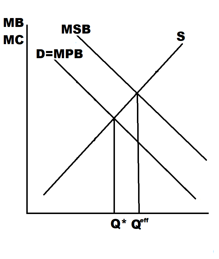
Figure 8.3: Illustration of Pigouvian tax
The equilibrium is the intersection of supply, marginal private cost, and demand, marginal private benefit. This is of course the allocation \(Q^*\).
But the efficient allocation is again the intersection of marginal social benefit and marginal private cost. We see that \(Q^{eff}\) is bigger than \(Q^*\). We have underproduction. The equilibrium is not efficient. Again, we have market failure.
The solution is a subsidy, a Pigouvian subsidy.
Why? Since the market participants do not take into consideration the extra external benefit, there is not enough stuff produced. How do we get the market to produce more? With a per unit subsidy that lowers someone’s private marginal cost.
But them the big question is:
- How to finance this subsidy?
- Which taxes to raise?
- Which other government programs to cut?
- Or should we just run a deficit?
After having explained positive and negative externalities, it is high time to state a formal definition of an externality.
An externality is present whenever any action causes a cost or a benefit to someone who is not involved in that action. That consequence could be positive or negative.
One qualification is in order:
Consider the following example: Imagine that IU cuts its incoming class down to 4000 students for a few years. We can safely predict that prices of apartments in Bloomington would fall. The single mom in Bloomington who is renting will be a beneficiary. But she has nothing to do with IU’s decision to cut enrollment.
We do not call this an externality. There is no inefficiency as in the above cases. The price will drop. But this price drop is simply a market signal.
With the enrollment drop, the demand for housing has dropped. If the demand has dropped, housing will be less scarce, and then we would expect, and we would want6 the price to drop.
8.4 Example
So far we have not specified at all how many people are influenced by the externality or what is the geographic reach of the eternal effect.
There are certain externalities that have a far reach and influence many people. Global climate change has global reach and reaches over 7 billion people.
Other externalities are severely limited in geographic reach and therefore also limited in the number of people impacted. Secondhand smoke is one of those examples. The Covid 19 externality is in some sense extremely limited in scope: 6 to 8 feet. That externality only increases its reach because of peoples’ mobility. The Chinese businessman who is infected can easily bring the virus to Northern Italy in January of 2020. The German family skiing in Northern Italy brings the bug back to Germany and from there it is off to the races to NYC, Miami, San Fran etc. The bug is mobile and has global reach because we are.
The bug is also very mobile because we are social creatures. We love to congregate in large groups, often indoors, for weddings, motorbike rallies, political election campaign events. The bug loves crowds, makes it easier to spread.
We will now study the case of an externality where the action by one person harms one other person. We can think of an upstream farmer/power plant who causes run-off into the river/the river water to warm up. Both actions damage the yield of a down steam fishery.
The situation is captured in Figure 8.4 here.
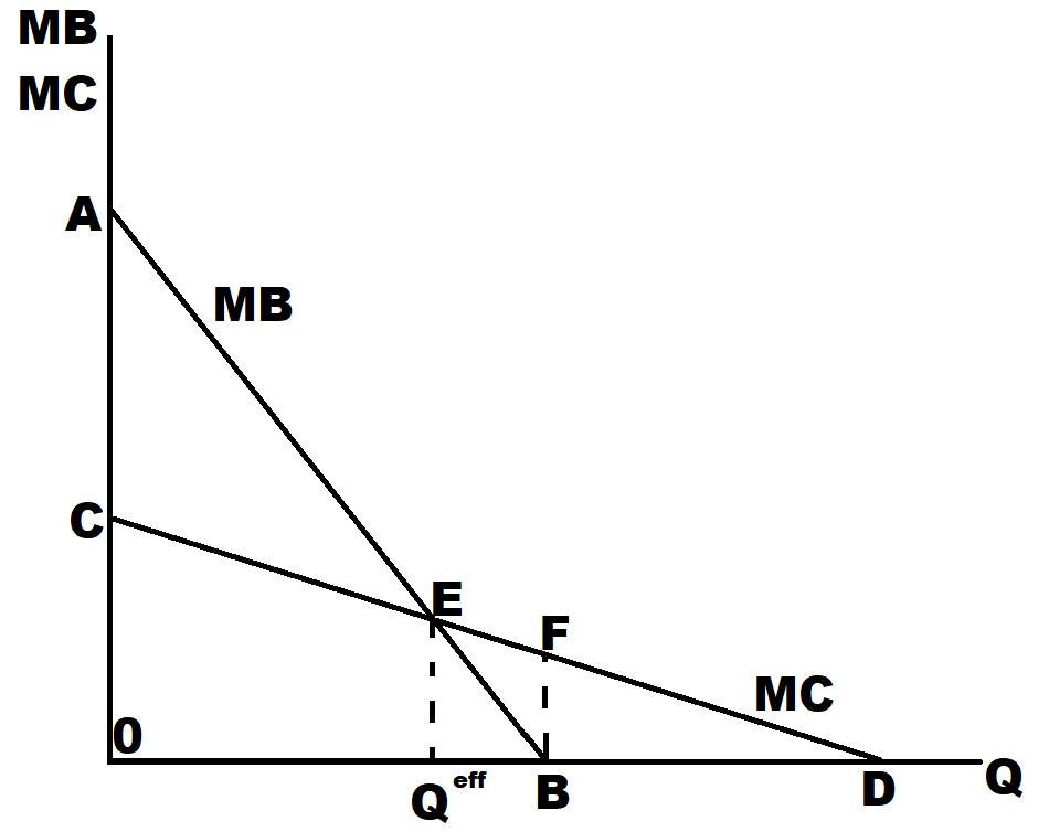
Figure 8.4: Externality
The line \(AB\) is the marginal benefit to the farmer, net of all costs. You can think of this as marginal profit, per unit of run-off generated. The profit maximizing point for the farmer is point \(B\), marginal profit is zero.
The line \(CD\) is the marginal cost to the downstream fishery. This is a cost caused by the farmer, his run-off, but it is incurred by the fishery. This is an external cost.
The efficient point is, as always, the point where marginal cost and marginal benefit intersect. It is the point marked \(Q^{eff}\).
How do we get to efficiency?
There are two ways to get there. And this might actually be quite surprising.
First, I give all the pollution rights to the farmer. The farmer may pollute as much as is in the farmer’s interest. In that case the farmer chooses point \(B\). How will the fishery react? The fishery will be better off at \(Q^{eff}\). It might be in the fisheries interest to coax the farmer to move to point \(E\).
Moving from point \(B\) to point \(E\) entails a loss to the farmer and a gain to the fishery.
The loss to the farmer is the area of the triangle \(Q^{eff}BE\).
The gain to the fishery is the area of the trapezoid \(Q^{eff}BFE\).
The gain to the fishery is bigger than the loss to the farmer.
Surely the fishery can make an offer to the farmer for a payment that is smaller than the fisheries gain and larger than the farmer’s loss.
This is like bargaining over how to split \(\$100\) between two people.
There is one fundamental difference: When two people have to split \(\$100\), they know the size of the pie is \(\$100\). The farmer is unlikely to know the cost imposed on the fishery. And the fishery is unlikely to know the benefits of the farmer. The two will have no idea how big their joint surplus really is. That can make things complicated.
Imagine you are bargaining with someone else about how to split an amount of money, but you think it is \(\$10\),000 and the other person thinks it is \(\$15,000\).
Instead of assigning property rights to the farmer, we could assign them to the fishery. The fishery would of course choose zero pollution. That is at point \(C\). In this case also, bargaining can get us to the efficient outcome. Getting from \(C\) to \(E\) is a loss to the fishery, but a gain to the farmer. The gain to the farmer is bigger than the loss to the fishery. The farmer can make an offer to the fishery and both will be at point \(E\).
8.5 Numerical Problems
-
Demand is given by P = 40 – Q. Supply is given by P = Q. The marginal external cost is given by 10.
A. Calculate the competitive equilibrium price and quantity.
B. Calculate the efficient price and quantity.
C. Calculate the deadweight loss of the externality.
D. Now imagine there is a per unit tax imposed on firms of 6. Calculate the competitive equilibrium price and quantity with this tax.
E. Calculate the deadweight loss of the externality with the tax. -
Demand is given by P = 10 -Q. Supply is given by P = Q. The marginal external benefit is given by 2.
A. Calculate the competitive equilibrium price and quantity.
B. Calculate the efficient price and quantity.
C. Calculate the deadweight loss of the externality.
D. How large would a per unit subsidy to the firms have to be so that the equilibrium price and quantity with the tax is efficient. Show your analysis. -
Imagine a situation of two producers like the farmer and the fishery. The farmer’s marginal benefit is given by MB = 20 – 2Q. The fishery’s marginal cost of the farmer’s action is given by MC = 15-Q.
A. Calculate the efficient point.
B. Assume all pollution rights are assigned to the farmer. Calculate the farmer’s best point. Calculate the fishery’s gain if they would move from the farmer’s best point to the efficient point. Calculate the farmer’s loss if they were to move from the farmer’s best point to the efficient point. Would it be in the best interest of the fishery to make a payment to the farmer to move to the efficient point? Would it be in the best interest of the farmer to accept it?
C. Repeat part b assuming the pollution rights are all assigned to the fishery. -
Imagine a situation of two producers like the farmer and the fishery. The farmer’s marginal benefit is given by MB = 20 – 2Q. The fishery’s marginal cost is given by MC = 10 – Q.
A. Calculate the efficient level of Q.
B. What kind of policy do you think is required to get to the efficient point in this situation. -
Imagine a situation of two producers like the farmer and the fishery. The farmer’s marginal benefit is given by MB = 10 – ½ Q. The fishery’s marginal cost is given by MC = 12 – Q.
A. Calculate the efficient level of Q. Hint: Some of you might consider this a bit of a trick question.
B. Repeat part a but assume that MC = 15 – Q.
C. What are the interpretations of the answers in parts a and b?